Safe Pareto Improvements for Delegated Game Playing

This article appeared in the journal Autonomous Agents and Multi-Agent Systems. An earlier, abbreviated version also appeared in the proceedings of AAMAS 2021.
 
 

$$\begin{array}{ccc} \textbf{Caspar Oesterheld} & &\textbf{Vincent Conitzer}\\ \texttt{Foundations of Cooperative AI Lab} & &\texttt{Foundations of Cooperative AI Lab}\\ \text{Computer Science Department} & &\text{Computer Science Department}\\ \text{Carnegie Mellon University} & &\text{Carnegie Mellon University}\\ \end{array}$$

Abstract

A set of players delegate playing a game to a set of representatives, one for each player. We imagine that each player trusts their respective representative’s strategic abilities. Thus, we might imagine that per default, the original players would simply instruct the representatives to play the original game as best as they can. In this paper, we ask: are there safe Pareto improvements on this default way of giving instructions? That is, we imagine that the original players can coordinate to tell their representatives to only consider some subset of the available strategies and to assign utilities to outcomes differently than the original players. Then can the original players do this in such a way that the payoff is guaranteed to be weakly higher than under the default instructions for all the original players? In particular, can they Pareto-improve without probabilistic assumptions about how the representatives play games? In this paper, we give some examples of safe Pareto improvements. We prove that the notion of safe Pareto improvements is closely related to a notion of outcome correspondence between games. We also show that under some specific assumptions about how the representatives play games, finding safe Pareto improvements is NP-complete.

Keywords: program equilibrium; delegation; bargaining; Pareto efficiency; smart contracts.

1 Introduction

Between Aliceland and Bobbesia lies a sparsely populated desert. Until recently, neither of the two countries had any interest in the desert. However, geologists have recently discovered that it contains large oil reserves. Now, both Aliceland and Bobbesia would like to annex the desert, but they worry about a military conflict that would ensue if both countries insist on annexing.

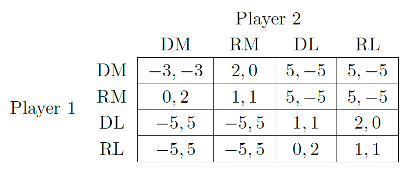
Table 1 models this strategic situation as a normal-form game. The strategy DM (short for “Demand with Military”) denotes a military invasion of the desert, demanding annexation. If both countries send their military with such an aggressive mission, the countries fight a devastating war. The strategy RM (for “Refrain with Military”) denotes yielding the territory to the other country, but building defenses to prevent an invasion of one’s current territories. Alternatively, the countries can choose to not raise a military force at all, while potentially still demanding control of the desert by sending only its leader (DL, short for “Demand with Leader”). In this case, if both countries demand the desert, war does not ensue. Finally, they could neither demand nor build up a military (RL). If one of the two countries has their military ready and the other does not, the militarized country will know and will be able to invade the other country. In gametheoretic terms, militarizing therefore strictly dominates not militarizing.

Instead of making the decision directly, the parliaments of Aliceland and Bobbesia appoint special commissions for making this strategic decision, led by Alice and Bob, respectively. The parliaments can instruct these representatives in various ways. They can explicitly tell them what to do – for example, Aliceland could directly tell Alice to play DM. However, we imagine that the parliaments trust the commissions’ judgments more than they trust their own and hence they might prefer to give an instruction of the type, “make whatever demands you think are best for our country” (perhaps contractually guaranteeing a reward in proportion to the utility of the final outcome). They might not know what that will entail, i.e., how the commissions decide what demands to make given that instruction. However – based on their trust in their representatives – they might still believe that this leads to better outcomes than giving an explicit instruction.

We will also imagine these instructions are (or at least can be) given publicly and that the commissions are bound (as if by a contract) to follow these instructions. In particular, we imagine that the two commissions can see each other’s instructions. Thus, in instructing their commissions, the countries play a game with bilateral precommitment. When instructed to play a game as best as they can, we imagine that the commissions play that game in the usual way, i.e., without further abilities to credibly commit or to instruct subcommittees and so forth.

It may seem that without having their parliaments ponder equilibrium selection, Aliceland and Bobbesia cannot do better than leave the game to their representatives. Unfortunately, in this default equilibrium, war is still a possibility. Even the brilliant strategists Alice and Bob may not always be able to resolve the difficult equilibrium selection problem to the same pure Nash equilibrium.

In the literature on commitment devices and in particular the literature on program equilibrium, important ideas have been proposed for avoiding such bad outcomes. Imagine for a moment that Alice and Bob will play a Prisoner’s Dilemma (Table 3) (rather than the Demand Game of Table 1). Then the default of (Defect, Defect) can be Pareto-improved upon. Both original players (Aliceland and Bobbesia) can use the following instruction for their representatives: “If the opponent’s instruction is equal to this instruction, Cooperate; otherwise Defect.” [33, 22, 46, Sect. 10.4, 55] Then it is a Nash equilibrium for both players to use this instruction. In this equilibrium, (Cooperate, Cooperate) is played and it is thus Pareto-optimal and Pareto-better than the default.

In cases like the Demand Game, it is more difficult to apply this approach to improve upon the default of simply delegating the choice. Of course, if one could calculate the expected utility of submitting the default instructions, then one could similarly commit the representatives to follow some (joint) mix over the Pareto-optimal outcomes ((RM, DM), (DM, RM), (RM, RM), (DL, DL), etc.) that Pareto-improves on the default expected utilities.¹ However, we will assume that the original players are unable or unwilling to form probabilistic expectations about how the representatives play the Demand Game, i.e., about what would happen with the default instructions. If this is the case, then this type of Pareto improvement on the default is unappealing.

The goal of this paper is to show and analyze how even without forming probabilistic beliefs about the representatives, the original players can Pareto-improve on the default equilibrium. We will call such improvements safe Pareto improvements (SPIs). We here briefly give an example in the Demand Game.

The key idea is for the original players to instruct the representatives to select only from {DL,RL}, i.e., to not raise a military. Further, they tell them to disvalue the conflict outcome without military (DL, DL) as they would disvalue the original conflict outcome of war in the default equilibrium. Overall, this means telling them to play the game of Table 2. (Again, we could imagine that the instructions specify Table 2 to be how Aliceland and Bobbesia financially reward Alice and Bob.) Importantly, Aliceland’s instruction to play that game must be conditional on Bobbesia also instructing their commission to play that game, and vice versa. Otherwise, one of the countries could profit from deviating by instructing their representative to always play DM or RM (or to play by the original utility function).

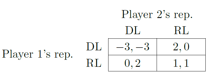
The game of Table 2 is isomorphic to the DM-RM part of the original Demand Game of Table 1. Of course, the original players know neither how the original Demand Game nor the game of Table 2 will be played by the representatives. However, since these games are isomorphic, one should arguably expect them to be played isomorphically. For example, one should expect that (RM,DM) would be played in the original game if and only if (RL, DL) would be played in the modified game. However, the conflict outcome (DM,DM) is replaced in the new game with the outcome (DL, DL). This outcome is harmless (Pareto-optimal) for the original players.

Contributions. Our paper generalizes this idea to arbitrary normal-form games and is organized as follows. In Section 2, we introduce some notation for games and multivalued functions that we will use throughout this paper. In Section 3, we introduce the setting of delegated game playing for this paper. We then formally define and further motivate the concept of safe Pareto improvements. We also define and give an example of unilateral SPIs. These are SPIs that require only one of the players to commit their representative to a new action set and utility function. In Section 3.2, we briefly review the concepts of program games and program equilibrium and show that SPIs can be implemented as program equilibria. In Section 4.2, we introduce a notion of outcome correspondence between games. This relation expresses the original players’ beliefs about similarities between how the representatives play different games. In our example, the Demand Game of Table 1 (arguably) corresponds to the game of Table 2 in that the representatives (arguably) would play (DM,DM) in the original game if and only if they play (DL, DL) in the new game, and so forth. We also show some basic results (reflexivity, transitivity, etc.) about the outcome correspondence relation on games. In Section 4.3 we show that the notion of outcome correspondence is central to deriving SPIs. In particular, we show that a game $\Gamma^s$ is an SPI on another game $\Gamma$ if and only if there is a Pareto-improving outcome correspondence relation between $\Gamma^s$ and $\Gamma$.

To derive SPIs, we need to make some assumptions about outcome correspondence, i.e., about which games are played in similar ways by representatives. We give two very weak assumptions of this type in Section 4.4. The first is that the representatives’ play is invariant under the removal of strictly dominated strategies. For example, we assume that in the Demand Game the representatives only play DM and RM. Moreover we assume that we could remove DL and RL from the game and the representatives would still play the same strategies as in the original Demand Game with certainty. The second assumption is that the representatives play isomorphic games isomorphically. For example, once DL and RL are removed for both players from the Demand Game, the Demand Game is isomorphic to the game in Table 2 such that we might expect them to be played isomorphically. In Section 4.5, we derive a few SPIs – including our SPI for the Demand Game – using these assumptions. Section 4.6 shows that determining whether there exists an SPI based on these assumptions is NP-complete. Section 5 considers a different setting in which we allow the original players to let the representatives choose from newly constructed strategies whose corresponding outcomes map arbitrarily onto feasible payoff vectors from the original game. In this new setting, finding SPIs can be done in polynomial time. We conclude by discussing the problem of selecting between different SPIs on a given game (Section 6) and giving some ideas for directions for future work (Section 7).

2 Preliminaries

We here give some basic game-theoretic definitions. We assume the reader to be familiar with most of these concepts and with game theory more generally.

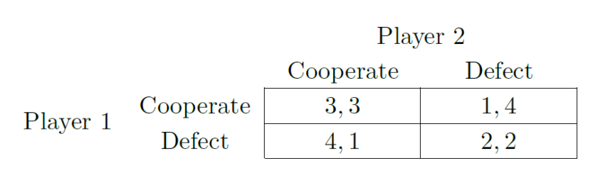
An $n$-player (normal-form) game is a tuple $(A,\mathbf{u})$ of a set $A=A_1\times ... \times A_n$ of (pure) strategy profiles (or outcomes) and a function $\mathbf{u}\colon A \rightarrow \mathbb{R}^n$ that assigns to each outcome a utility for each player. The Prisoner's Dilemma shown in Table 3 is a classic example of a game. The Demand Game of Table 1 is another example of a game that we will use throughout this paper.

Instead of $(A,\mathbf{u})$ we will also write $(A_1,...,A_n,u_1,...,u_n)$. We also write $A_{-i}$ for $\times_{j\neq i} A_i$, i.e., for the Cartesian product of the action sets of all players other than $i$. We similarly write $\mathbf{u}_{-i}$ and $\mathbf{a}_{-i}$ for vectors containing utility functions and actions, respectively, for all players but $i$. If $u_i$ is a utility function and $\mathbf{u}_{-i}$ is a vector of utility functions for all players other than $i$, then (even if $i\neq 1$) we use $(u_i,\mathbf{u}_{-i})$ for the full vector of utility functions where Player $i$ has utility function $u_i$ and the other players have utility functions as specified by $\mathbf{u}_{-i}$. We use $(A_i,A_{-i})$ and $(a_i,\mathbf{a}_{-i})$ analogously.

We say that $a_i\in A_i$ strictly dominates $a_i'\in A_i$ if for all $a_{-i}\in A_{-i}$, $u_i(a_i,a_{-i})>u_i(a_{i}',a_{-i})$. For example, in the Prisoner's Dilemma, Defect strictly dominates Cooperate for both players. As noted earlier, $\mathrm{DM}$ and $\mathrm{RM}$ strictly dominate $\mathrm{DL}$ and $\mathrm{RL}$ for both players.

For any given game $\Gamma=(A,\mathbf{u})$, we will call any game $\Gamma'=(A',\mathbf{u}')$ a subset game of $\Gamma$ if $A_i'\subseteq A_i$ for $i=1,...,n$. Note that a subset game may assign different utilities to outcomes than the original game. For example, the game of Table 2 is a subset game of the Demand Game.

We say that some utility vector $\mathbf{y}\in \mathbb{R}^n$ is a Pareto improvement on (or is Pareto-better than) $\mathbf{y}'\in \mathbb{R}^n$ if $y_i\geq y_i'$ for $i=1,...,n$. We will also denote this by $\mathbf{y}\geq \mathbf{y}'$. Note that, contrary to convention, we allow $\mathbf{y}=\mathbf{y}'$. Whenever we require one of the inequalities to be strict, we will say that $\mathbf{y}$ is a strict Pareto improvement on $\mathbf{y}'$. In a given game, we will also say that an outcome $\mathbf{a}$ is a Pareto improvement on another outcome $\mathbf{a}'$ if $\mathbf{u}(\mathbf{a}) \geq \mathbf{u}(\mathbf{a}')$. We say that $\mathbf{y}$ is Pareto-optimal or Pareto-efficient relative to some $S\subset \mathbb{R}^n$ if there is no element of $S$ that strictly Pareto-dominates $\mathbf{y}$.

Let $\Gamma=(A,\mathbf{u})$ and $\Gamma'=(A',\mathbf{u}')$ be two $n$-player games. Then we call an $n$-tuple of functions $\Phi=\left(\Phi_i\colon A_i\rightarrow A_i'\right)_{i=1,...,n}$ a (game) isomorphism between $\Gamma$ and $\Gamma'$ if there are vectors $\boldsymbol{\lambda}\in\mathbb{R}_{+}^n$ and $\mathbf{c}\in\mathbb{R}^n$ such that

$$\begin{equation*} u_i(a_1,...,a_n) = \lambda_i u_i'(\Phi_1(a_1),...,\Phi_n(a_n))+c_i \end{equation*}$$

for all $\mathbf{a}\in A$ and $i=1,...,n$. If there is an isomorphism between $\Gamma$ and $\Gamma'$, we call $\Gamma$ and $\Gamma'$ isomorphic. For example, if we let $\Gamma$ be the Demand Game and $\Gamma^s$ the subset game of Table 2, then $(\{\mathrm{DM},\mathrm{RM}\},\{\mathrm{DM},\mathrm{RM}\},\mathbf{u})$ is isomorphic to $\Gamma^s$ via the isomorphism $\Phi$ with $\Phi_i(\mathrm{DM})=\mathrm{DL}$ and $\Phi_i(\mathrm{RM})=\mathrm{RL}$ and the constants $\boldsymbol{\lambda}=(1,1)$ and $\mathbf{c}=(0,0)$.

3 Delegation and safe Pareto improvements

We consider a setting in which a given game $\Gamma$ is played through what we will call representatives. For example, the representatives could be humans whose behavior is determined or incentivized by some contract à la the principal–agent literature [28]. Our principals’ motivation for delegation is the same as in that literature (namely, the agent being in a better (epistemic) position to make the choice). However, the main question asked by the principal–agent literature is how to deal with agents that have their own preferences over outcomes, by constraining the agent’s choice [e.g. 21, 25], setting up appropriate payment schemes [e.g. 23, 29, 37, 53], etc. In contrast, we will throughout this paper assume that the agent has no conflicting incentives.

We imagine that one way in which the representatives can be instructed is to in turn play a subset game $\Gamma^s=(A_1^s\subseteq A_1,...,A_n^s\subseteq A_n,\mathbf{u}^s)$ of the original game, without necessarily specifying a strategy or algorithm for solving such a game. We emphasize, again, that $\mathbf{u}^s$ is allowed to be a vector of entirely different utility functions. For any subset game $\Gamma^s$, we denote by $\Pi(\Gamma^s)$ the outcome that arises if the representatives play the subset game $\Gamma^s$ of $\Gamma$. Because it is unclear what the right choice is in many games, the original players might be uncertain about $\Pi(\Gamma^s)$. We will therefore model each $\Pi(\Gamma^s)$ as a random variable. We will typically imagine that the representatives play $\Gamma$ in the usual simultaneous way, i.e., that they are not able to make further commitments or delegate again. For example, we imagine that if $\Gamma$ is the Prisoner's Dilemma, then $\Pi(\Gamma)=(\mathrm{Defect},\mathrm{Defect})$ with certainty.

The original players trust their representatives to the extent that we take $\Pi(\Gamma)$ to be a default way for the game to played for any $\Gamma$. That is, by default the original players tell their representatives to play the game as given. For example, in the Demand Game, it is not clear what the right action is. Thus, if one can simply delegate the decision to someone with more relevant expertise, that is the first option one would consider.

We are interested in whether and how the original players can jointly Pareto-improve on the default. Of course, one option is to first compute the expected utilities under default delegation, i.e., to compute $\mathbb{E}\left[\mathbf{u}(\Pi(\Gamma))\right]$. The players could then let the representatives play a distribution over outcomes whose expected utilities exceed the default expected utilities. However, this is unrealistic if $\Gamma$ is a complex game with potentially many Nash equilibria. For one, the precise point of delegation is that the original players are unable or unwilling to properly evaluate $\Gamma$. Second, there is no widely agreed upon, universal procedure for selecting an action in the face of equilibrium selection problems. In such cases, the original players may in practice be unable to form a probability distribution over $\Pi(\Gamma)$. This type of uncertainty is sometimes referred to as Knightian uncertainty, following Knight's [26] distinction between the concepts of risk and uncertainty.

We address this problem in a typical way. Essentially, we require of any attempted improvement over the default that it incurs no regret in the worst-case. That is, we are interested in subset games $\Gamma^s$ that are Pareto improvements with certainty under weak and purely qualitative assumptions about $\Pi$.² In particular, in Section 4.4, we will introduce the assumptions that the representatives do not play strictly dominated actions and play isomorphic games isomorphically.

Definition 1. Let $\Gamma^s$ be a subset game of $\Gamma$. We say $\Gamma^s$ is a safe Pareto improvement (SPI) on $\Gamma$ if $\mathbf{u}(\Pi(\Gamma^s))\geq \mathbf{u}(\Pi(\Gamma))$ with certainty. We say that $\Gamma^s$ is a strict SPI if furthermore, there is a player $i$ s.t. $u_i(\Pi(\Gamma^s))>u_i(\Pi(\Gamma^s))$ with positive probability.

For example, in the introduction we have argued that the subset game in Table 2 is a strict SPI on the Demand Game (Table 1). Less interestingly, if we let $\Gamma=(A,\mathbf{u})$ be the Prisoner's Dilemma (Table 3), then we would expect $(\{\mathrm{Cooperate}\},\{\mathrm{Cooperate}\},\mathbf{u})$ to be an SPI on $\Gamma$. After all, we might expect that $\Pi(\Gamma)=(\mathrm{Defect},\mathrm{Defect})$ with certainty, while it must be

$$\Pi(\{\mathrm{Cooperate}\},\{\mathrm{Cooperate}\},\mathbf{u})= (\mathrm{Cooperate},\mathrm{Cooperate})$$

with certainty, for lack of alternatives. Both players prefer mutual cooperation over mutual defection.

3.1 Unilateral safe Pareto Improvements

Both SPIs given above require both players to let their representatives choose from restricted strategy sets to maximize something other than the original player's utility function.

Definition 2. We will call a subset game $\Gamma^s=(A^s,\mathbf{u}^s)$ of $\Gamma=(A,\mathbf{u})$ unilateral if for all but one $i\in \{1,...,n\}$ it holds that $A_i^s=A_i$ and $u_i^s=u_i$. Consequently, if a unilateral subset game $\Gamma^s$ of $\Gamma$ is also an SPI for $\Gamma$, we call $\Gamma^s$ a unilateral SPI.

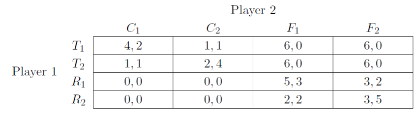
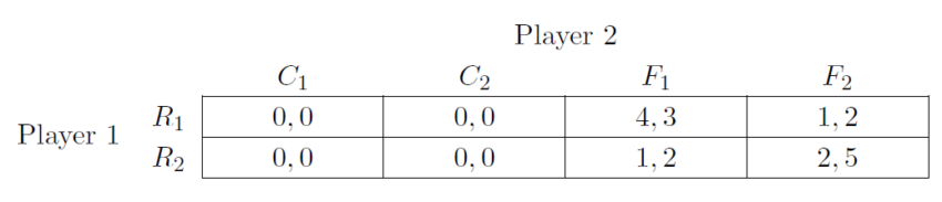
We now give an example of a unilateral SPI using the Complicated Temptation Game. (We give the not-so-complicated Temptation Game – in which we can only give a trivial example of SPIs – in Section 4.5.) Two players each deploy a robot. Each of the robots faces two choices in parallel. First, each can choose whether to work on Project 1 or Project 2. Player 1 values Project 1 higher and Player 2 values Project 2 higher, but the robots are more effective if they work on the same project. To complete the task, the two robots need to share a resource. Robot 2 manages the resource and can choose whether to control Robot 1’s access tightly (e.g., by frequently checking on the resource, or requiring Robot 1 to demonstrate a need for the resource) or give Robot 1 relatively free access. Controlling access tightly decreases the efficiency of both robots, though the exact costs depend on which projects the robots are working on. Robot 1 can choose between using the resource as intended by Robot 2; or give in to the temptation of trying to steal as much of the resource as possible to use it for other purposes. Regardless of what Robot 2 does (in particular, regardless of whether Robot 2 controls access or not), Player 1 prefers trying to steal. In fact, if Robot 2 controls access and Robot 1 refrains from theft, they never get anything done. Given that Robot 1 tries to steal, Player 2 prefers his Robot 2 to control access. As usual we assume that the original players can instruct their robots to play arbitrary subset games of $\Gamma$ (without specifying an algorithm for solving such a game) and that they can give such instructions conditional on the other player providing an analogous instruction.

We formalize this game as a normal-form game in Table 4. Each action consists of a number and letter. The number indicates the project that the agent pursues. The letters indicates the agent’s policy towards the resource. In Player 2’s action labels, C indicates tight control over the resource, while F indicates free access. In Player 1’s action labels, T indicates giving in to the temptation to steal as much of the resource as possible, while R indicates refraining from doing so.

Player 1 has a unilateral SPI in the Complicated Temptation Game. Intuitively, if Player 1 commits to refrain, then Player 2 need not control the use of the resource. Thus, inefficiencies from conflict over the resource are avoided. However, Player 1’s utilities in the resulting game of choosing between projects 1 and 2 are not isomorphic to the original game of choosing between projects 1 and 2. The players might therefore worry that this new game will result in a worse outcome for them. For example, Player 2 might worry that in this new game the project 1 equilibrium ($T_1, F_1$) becomes more likely than the project 2 equilibrium. To address this, Player has to commit her representative to a different utility function that makes this new game isomorphic to the original game.

We now describe the unilateral SPI in formal detail. Player 1 can commit her representative to play only from $R_1$ and $R_2$ and to assign utilities $u^s_1(R_1,F_1)=u_1(T_1,C_1)=4$, $u^s_1(R_1,F_2)=u_1(T_1,C_2)=1$, $u^s_1(R_2,F_1)=u_1(T_2,C_1)=1$, and $u^s_1(R_2,F_2)=u_1(T_2,C_2)=2$; otherwise $u_1^s$ does not differ from $u_1$. The resulting SPI is given in Table 5. In this subset game, Player 2's representative – knowing that Player 1's representative will only play from $R_1$ and $R_2$ – will choose from $F_1$ and $F_2$ (since $F_1$ and $F_2$ strictly dominate $C_1$ and $C_2$ in Table 5). Now notice that the remaining subset game is isomorphic to the $(\{T_1,T_2\},\{C_1,C_2\})$ subset game of the original Complicated Temptation Game, where $T_1$ maps to $R_1$ and $T_2$ maps to $R_2$ for both Player 1, and $C_1$ maps to $F_1$ and $C_2$ maps to $F_2$ for Player 2. Player 1's representative's utilities have been set to be the same between the two; and Player 2's utilities happen to be the same up to a constant ($1$) between the two subset games. Thus, we might expect that if $\Pi(\Gamma)=(T_1,C_1)$, then $\Pi(\Gamma^s)=(R_1,F_1)$, and so on. Finally, notice that $\mathbf{u}(R_1,F_1)\geq \mathbf{u}(T_1,C_1)$ and so on. Hence, Table 5 is indeed an SPI on the Complicated Temptation Game.

 

Such unilateral changes are particularly interesting because they only require one of the players to be able to credibly delegate. That is, it is enough for a single player to instruct their representative to choose from a restricted action set to maximize a new utility function. The other players can simply instruct their representatives to play the game in the normal way (i.e., maximizing the respective players' original utility functions without restrictions on the action set). In fact, we may also imagine that only one player $i$ delegates at all, while the other players choose an action themselves, after observing Player $i$'s instruction to her representative.

One may object that in a situation where only one player can credibly commit and the others cannot, the player who commits can simply play the meta game as a standard unilateral commitment (Stackelberg) game [as studied by, e.g., 11, 52, 59] or perhaps as a first mover in a sequential game (as solved by subgame-perfect equilibrium), without bothering with any (safe) Pareto conditions, i.e., without ensuring that all players are guaranteed a utility at least as high as their default $\mathbf{u}(\Pi(\Gamma))$. For example, in the Complicated Temptation Game, Player 1 could simply commit her representative to play $R_1$ if she assumes that Player 2's representative will be instructed to best respond.

The Stackelberg sequential play perspective is appropriate in many cases. However, we think that in many cases the player with fine-grained commitment ability cannot assume that the other players' representatives will simply best respond. Instead, players often need to consider the possibility of a hostile response if their commitment forces an unfair payoff on the other players. In such cases, unilateral SPIs are relevant.

The Ultimatum game is a canonical example in which standard solution concepts of sequential play fail to predict human behavior. In this game, subgame-perfect equilibrium has the second-moving player walk away with arbitrarily close to nothing. However, experiments show that people often resolve the game to an equal split, which is the symmetric equilibrium of the simultaneous version of the game [38].

A policy of retaliating for unfair payoffs imposed by a first mover's commitments can arise in a variety of ways within standard game-theoretic models. For one, we may imagine a scenario in which only one Player has the fine-grained commitment and delegation abilities needed for SPIs but that the other players can still credibly commit their representatives to retaliate against any “commitment trickery” that clearly leaves them worse off. We may also imagine that other players or representatives come into the scenario having already made such commitments. For example, many people appear credibly committed by intuitions about fairness and retributivist instincts and emotions [see, e.g., 44, Chapter 6, especially the section “The Doomsday Machine”]. Perhaps these features of human psychology allow human second players in the Ultimatum game empirically outperform subgame-perfect equilibrium. Second, we may imagine that the players who cannot commit are subject to reputation effects. Then they might want to build a reputation of resisting coercion. In contrast, it is beneficial to have a reputation of accepting SPIs on whatever game would have otherwise been played.

3.2 Implementing safe Pareto improvements as program equilibria

 

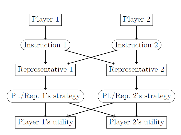
So far, we have been vague about the details of the strategic situation that the original players face in instructing their representatives. From what sets of actions can they choose? How can they jointly let the representatives play some new subset game $\Gamma^s$? Are SPIs Nash equilibria of the meta game played by the original players? If I instruct my representative to play the SPI of Table 2 in the Demand Game, could my opponent not instruct her representative to play $\mathrm{DM}$?

In this section, we briefly describe one way to fill this gap by discussing the concept of program games and program equilibrium [46, Sect. 10.4, 55, 15, 5, 13, 36]. This section is essential to understanding why SPIs (especially omnilateral ones) are relevant. However, the remaining technical content of this paper does not rely on this section and the main ideas presented here are straightforward from previous work. We therefore only give an informal exposition. For formal detail, see Appendix A.

For any game $\Gamma=(A,\mathbf{u})$, the program equilibrium literature considers the following meta game. First, each player $i$ writes a computer program. Each program then receives as input a vector containing everyone else's chosen program. Each player $i$'s program then returns an action from $A_i$, player $i$'s set of actions in $\Gamma$. Together these actions then form an outcome $\mathbf{a}\in A$ of the original game. Finally, the utilities $\mathbf{u}(\mathbf{a})$ are realized according to the utility function of $\Gamma$. The meta game can be analyzed like any other game. Its Nash equilibria are called program equilibria. Importantly, the program equilibria can implement payoffs not implemented by any Nash equilibria of $\Gamma$ itself. For example, in the Prisoner’s Dilemma, both players can submit a program that says: “If the opponent’s chosen computer program is equal to this computer program, Cooperate; otherwise Defect.” [33, 22, 46, Sect. 10.4, 55] This is a program equilibrium which implements mutual cooperation.

In the setting for our paper, we similarly imagine that each player $i$ can write a program that in turn chooses from $A_i$. However, the types of programs that we have in mind here are more sophisticated than those typically considered in the program equilibrium literature. Specifically we imagine that the programs are executed by intelligent representatives who are themselves able to competently choose an action for player $i$ in any given game $\Gamma^s$, without the original player having to describe how this choice is to be made. The original player may not even understand much about this program other than that it generally plays well. Thus, in addition to the elementary instructions used in a typical computer program (branches, comparisons, arithmetic operations, return, etc.), we allow player $i$ to use instructions of type “Play $\Pi_i(\Gamma^s)$” in the program she submits. This instruction lets the representative choose and return an action for the game $\Gamma^s$. Apart from the addition of this instruction type, we imagine the set of instructions to be the same as in the program equilibrium literature. To jointly let the representatives play, e.g., the SPI $\Gamma^s$ of Table 2 on the Demand Game of Table 1, the representatives can both use an instruction that says, “If the opponent's chosen program is equal to this one, play $\Pi_i(\Gamma^s)$; otherwise play $\mathrm{DM}$”. Assuming some minimal rationality requirements on the representatives (i.e., on how the representative resolves the “play $\Pi_i(\Gamma^s)$” instruction), this is a Nash equilibrium. Figure 1 illustrates how (in the two-player case) the meta game between the original players is intended to work.

For illustration consider the following two real-world instantiations of this setup. First, we might imagine that the original players hire human representatives. Each player specifies, e.g., via monetary incentives, how she wants her representative to act by some contract. For example, a player might contract her representative to play a particular action; or she might specify in her contract a function ($u_i^s$) over outcomes according to which she will pay the representative after an outcome is obtained. Moreover, these contracts might refer to one another. For example, Player 1's contract with her representative might specify that if Player 2 and his representative use an analogous contract, then she will pay her representative according to Table 2. As a second, more futuristic scenario, you could imagine that the representatives are software agents whose goals are specified by so-called smart contracts, i.e., computer programs implemented on a blockchain to be publicly verifiable [8, 47].

To justify our study of SPIs, we prove that every SPI is played in some program equilibrium:

Theorem 1. Let $\Gamma$ be a game and $\Gamma^s$ be an SPI of $\Gamma$. Now consider a program game on $\Gamma$, where each player $i$ can choose from a set of computer programs that output actions for $\Gamma$. In addition to the normal kind of instructions, we allow the use of the command "play $\Pi_i(\Gamma')$" for any subset game $\Gamma'$ of $\Gamma$. Finally, assume that $\Pi(\Gamma)$ guarantees each player $i$ at least that player's minimax utility (a.k.a. threat point) in the base game $\Gamma$. Then $\Pi(\Gamma^s)$ is played in a program equilibrium, i.e., in a Nash equilibrium of the program game.

We prove this in Appendix A.

As an alternative to having the original players choose contracts separately, we could imagine the use of jointly signed contracts which only come into effect once signed by all players [cf. 24, 34]. Another approach to bilateral commitment was pursued by Raub [45] based on earlier work by Sen [51]. Raub and Sen use preference modification as a mechanism for commitment. For example, in the Prisoner’s Dilemma, each player can separately instruct their representative to prefer cooperating over defecting if and only if the opponent also cooperates. If both players use this instruction, then mutual cooperation becomes the unique Pareto-optimal Nash equilibrium. On the other hand, if only one player instructs their representative to adopt these preferences and the other maintains the usual Prisoner’s Dilemma preferences, the unique equilibrium remains mutual defection. Thus, the preference modification is used to commit to cooperating conditional on the other player making an analogous commitment. Because this is slightly confusing in the context of our work – seeing as our work involves both modifying one’s preferences and mutual commitment, but generally without using the former as a means to the latter – we discuss Raub’s and Sen’s work and its relation to ours in more detail in Appendix B.

4 Safe Pareto improvements through outcome correspondence

4.1 Multivalued functions

For sets $M$ and $N$, a multi-valued function $\Phi\colon M\multimap N$ is a function which maps each element $m\in M$ to a set $\Phi(m)\subseteq N$. For a subset $Q\subseteq M$, we define

$$\begin{equation*} \Phi(Q)\coloneqq \bigcup_{m\in Q} \Phi(m). \end{equation*}$$

Note that $\Phi(Q)\subseteq N$ and that $\Phi(\emptyset)=\emptyset$. For any set $M$, we define the identity function $\mathrm{id}_M\colon M\multimap M\colon m\rightarrow \{ m \}$. Also, for two sets $M$ and $N$, we define $\mathrm{all}_{M,N}\colon M \multimap N\colon m \mapsto N$. We define the inverse

$$\begin{equation*} \Phi^{-1}\colon N \multimap M \colon n \mapsto \{ m \in M \mid n\in \Phi(m) \}. \end{equation*}$$

Note that $\Phi^{-1}(\emptyset)=\emptyset$ for any multi-valued function $\Phi$. For sets $M$, $N$ and $Q$ and functions $\Phi\colon M\multimap N$ and $\Psi\colon N \multimap Q$, we define the composite $\Psi \circ \Phi \colon M \multimap Q \colon m \mapsto \Psi(\Phi(m))$. As with regular functions, composition of multi-valued functions is associative. We say that $\Phi\colon M\multimap N$ is single-valued if $|\Phi(m)|=1$ for all $m\in M$. Whenever a multi-valued function is single-valued, we can apply many of the terms for regular functions. For example, we will take injectivity, surjectivity, and bijectivity for single-valued functions to have the usual meaning. We will never apply these notions to non-single-valued functions.

4.2 Outcome correspondence between games

In this section, we introduce a notion of outcome correspondence, which we will see is essential to constructing SPIs.

Definition 3. Consider two games $\Gamma=(A_1,...,A_n,\mathbf{u})$ and $\Gamma'=(A_1',...,A_n',\mathbf{u}')$. We write $\Gamma\sim_{\Phi} \Gamma'$ for $\Phi\colon A \multimap A'$ if $\Pi(\Gamma')\in \Phi(\Pi(\Gamma))$ with certainty.

Note that $\Gamma\sim_{\Phi} \Gamma'$ is a statement about $\Pi$, i.e., about how the representatives choose. Whether such a statement holds generally depends on the specific representatives being used. In Section 4.4, we describe two general circumstances under which it seems plausible that $\Gamma\sim_{\Phi} \Gamma'$. For example, if two games $\Gamma$ and $\Gamma'$ are isomorphic, then one might expect $\Gamma\sim_{\Phi} \Gamma'$, where $\Phi$ is the isomorphism between the two games.

We now illustrate this notation using our discussion from the Demand Game. Let $\Gamma$ be the Demand Game of Table 1. First, it seems plausible that $\Gamma$ is in some sense equivalent to $\Gamma'$, where $\Gamma'=(\{\mathrm{DM},\mathrm{RM},\mathrm{u})$ is the game that results from removing $\mathrm{DL}$ and $\mathrm{RL}$ for both players from $\Gamma$. Again, strict dominance could be given as an argument. We can now formalize this as $\Gamma \sim_{\Phi} \Gamma'$, where $\Phi(a_1,a_2)=\{(a_1,a_2)\}$ if $a_1,a_2\in \{\mathrm{DM},\mathrm{RM}\}$ and $\Phi(a_1,a_2)=\emptyset$ otherwise. Next, it seems plausible that $\Gamma'\sim_{\Psi} \Gamma^s$, where $\Gamma^s$ is the game of Table 2 and $\Psi$ is the isomorphism between $\Gamma'$ and $\Gamma^s$.

We now state some basic facts about the relation $\sim$, many of which we will use throughout this paper.

Lemma 2. Let $\Gamma=(A,\mathbf{u})$, $\Gamma'=(A',\mathbf{u}')$, $\hat \Gamma=(\hat A,\hat{\mathbf{u}})$ and $\Phi,\Xi \colon A\multimap A'$, $\Psi\colon A' \multimap \hat A$.

1. Reflexivity: $\Gamma \sim_{\mathrm{id}_A} \Gamma$, where $\mathrm{id}_{A} \colon A \multimap A \colon \mathbf{a} \mapsto \{\mathbf{a}\}$.
2. Symmetry: If $\Gamma\sim_{\Phi} \Gamma'$, then $\Gamma' \sim_{\Phi^{-1}} \Gamma$.
3. Transitivity: If $\Gamma\sim_{\Phi} \Gamma'$ and $\Gamma'\sim_{\Psi} \hat \Gamma$, then $\Gamma\sim_{\Psi \circ \Phi} \hat \Gamma$.
4. If $\Gamma\sim_{\Phi} \Gamma'$ and $\Phi(\mathbf{a})\subseteq \Xi (\mathbf{a})$ for all $\mathbf{a}\in A$, then $\Gamma\sim_{\Xi} \Gamma'$.
5. $\Gamma\sim_{\mathrm{all}_{A,A'}} \Gamma'$, where $\mathrm{all}_{A,A'} \colon A \multimap A' \colon \mathbf{a} \mapsto A'$.
6. If $\Gamma\sim_{\Phi} \Gamma'$ and $\Phi(\mathbf{a})=\emptyset$, then $\Pi(\Gamma)\neq \mathbf{a}$ with certainty.
7. If $\Gamma\sim_{\Phi} \Gamma'$ and $\Phi^{-1}(\mathbf{a}')=\emptyset$, then $\Pi(\Gamma')\neq \mathbf{a}'$ with certainty.

Proof. 1. By reflexivity of equality, $\Pi(\Gamma)=\Pi(\Gamma)$ with certainty. Hence, $\Pi(\Gamma)\in \mathrm{id}_A(\Pi(\Gamma))$ by definition of $\mathrm{id}_A$. Therefore, $\Gamma\sim_{\mathrm{id}_A} \Gamma$ by definition of $\sim$, as claimed.

2. $\Gamma\sim_{\Phi} \Gamma'$ means that $\Pi(\Gamma')\in \Phi(\Pi(\Gamma))$ with certainty. Thus,

$$\begin{equation*} \Pi(\Gamma)\in \{ \mathbf{a}{\in} A\mid \Pi(\Gamma'){\in} \Phi(\mathbf{a}) \} =\Phi^{-1}(\Pi(\Gamma')), \end{equation*}$$

where equality is by the definition of the inverse of multi-valued functions. We conclude (by definition of $\sim$) that $\Gamma'\sim_{\Phi^{-1}} \Gamma$ as claimed.

3. If $\Gamma \sim _{\Phi} \Gamma'$, $\Gamma'\sim_{\Psi} \hat \Gamma$, then by definition of $\sim$, (i) $\Pi(\Gamma')\in \Phi(\Pi(\Gamma))$ and (ii) $\Pi(\hat\Gamma)\in \Psi(\Pi(\Gamma'))$, both with certainty. The former (i) implies $\{ \Pi(\Gamma')\} \subseteq \Phi(\Pi(\Gamma))$. Hence,

$$\begin{equation*} \Psi(\Pi(\Gamma'))=\Psi(\{\Pi(\Gamma')\}) \subseteq \Psi(\Phi(\Pi(\Gamma))). \end{equation*}$$

With ii, it follows that $\Pi(\hat \Gamma)\in \Psi(\Phi(\Pi(\Gamma)))$ with certainty. By definition, $\Gamma \sim_{\Psi\circ\Phi}\hat \Gamma$ as claimed.

4. It is

$$\begin{equation*} \Pi(\Gamma')\in \Phi(\Pi(\Gamma)) \subseteq \Xi(\Pi(\Gamma)) \end{equation*}$$

with certainty. Thus, by definition $\Gamma\sim_{\Xi} \Gamma'$.

5. By definition of $\Pi$, it is $\Pi(\Gamma')\in A'$ with certainty. By definition of $\mathrm{all}_{A,A'}$, it is $\mathrm{all}_{A,A'}(\Pi(\Gamma))=A'$ with certainty. Hence, $\Pi(\Gamma')\in \mathrm{all}_{A,A'} (\Pi(\Gamma))$ with certainty. We conclude that $\Gamma\sim_{\mathrm{all}_{A,A'}}\Gamma'$ as claimed.

6. With certainty, $\Pi(\Gamma')\in \Phi(\Pi(\Gamma))$ (by assumption). Also, with certainty $\Pi(\Gamma')\notin\emptyset$. Hence, $\Phi(\Pi(\Gamma))\neq \emptyset$ with certainty. We conclude that $\Pi(\Gamma)\neq \mathbf{a}$ with certainty.

7. If $\Gamma\sim_{\Phi}\Gamma'$, then by reflexivity of $\sim$ (Lemma 2.1) $\Gamma'\sim_{\Phi^{-1}}\Gamma$. If $\Phi^{-1}(\mathbf{a}')=\emptyset$, then by Lemma 2.6, $\Pi(\Gamma')\neq \mathbf{a}'$ with certainty.

Items 1-3 show that $\sim$ has properties resembling those of an equivalence relation. Note, however, that since $\sim$ is not a binary relationship, $\sim$ itself cannot be an equivalence relation in the usual sense. We can construct equivalence relations, though, by existentially quantifying over the multivalued function. For example, we might define an equivalence relation $R$ on games, where $(\Gamma,\Gamma')\in R$ if and only if there is a single-valued bijection $\Phi$ such that $\Gamma\sim_{\Phi} \Gamma'$.³

Item 4 states that if we can make an outcome correspondence claim less precise, it will still hold true. Item 5 states that in the extreme, it is always $\Gamma \sim_{\mathrm{all}_{A,A'}} \Gamma'$, where $\mathrm{all}_{A,A'}$ is the trivial, maximally imprecise outcome correspondence function that confers no information. Item 6 shows that $\sim$ can be used to express the elimination of outcomes, i.e., the belief that a particular outcome (or strategy) will never occur.

Besides an equivalence relation, we can also use $\sim$ with quantification over the respective outcome correspondence function to construct (non-symmetric) preorders over games, i.e., relations that are transitive and reflexive (but not symmetric or antisymmetric). Most importantly, we can construct a preorder $\succeq$ on games where $\Gamma \succeq \Gamma'$ if $\Gamma \sim _{\Phi} \Gamma'$ for a $\Phi$ that always increases every player's utilities.

4.3 A theorem connecting outcome correspondence with safe Pareto improvements

We now show that as advertised, outcome correspondence is closely tied to SPIs. The following theorem shows not only how outcome correspondences can be used to find (and prove) SPIs. It also shows that any SPI requires an outcome correspondence relation via a Pareto-improving correspondence function.

Definition 4. Let $\Gamma=(A,\mathbf{u})$ be a game and $\Gamma^s = (A^s,\mathbf{u}^s)$ be a subset game of $\Gamma$. Further let $\Phi\colon A\rightarrow A^s$ be such that $\Gamma\sim_{\Phi} \Gamma'$. We call $\Phi$ a Pareto-improving outcome correspondence (function) if $\mathbf{u}(\mathbf{a}^s)\geq \mathbf{u}(\mathbf{a})$ for all $\mathbf{a}\in A$ and all $\mathbf{a}^s\in \Phi(\mathbf{a})$.

Theorem 3. Let $\Gamma=(A,\mathbf{u})$ be a game and $\Gamma^s = (A^s,\mathbf{u}^s)$ be a subset game of $\Gamma$. Then $\Gamma ^s$ is an SPI on $\Gamma$ if and only if there is a Pareto-improving outcome correspondence from $\Gamma$ to $\Gamma^s$.

Proof. $\Leftarrow$: By definition, $\Pi(\Gamma ^s )\in \Phi(\Pi(\Gamma ))$ with certainty. Hence, for $i=1,2$,

$$\begin{equation*} u_i(\Pi(\Gamma ^s))\in u_i(\Phi(\Pi(\Gamma ))) \end{equation*}$$

with certainty. Hence, by assumption about $\Phi$, with certainty, $u_i(\Pi(\Gamma ^s))\geq u_i(\Pi(\Gamma))$.

$\Rightarrow$: Assume that $u_{i} (\Pi(\Gamma)) \geq u_i(\Pi(\Gamma^s))$ with certainty for $i=1,2$. We define

$$\begin{equation*} \Phi\colon A\rightarrow A ^s\colon \mathbf{a} \mapsto \left\{ \mathbf{a}^s\in A^s \mid \mathbf{u}(\mathbf{a}^s) \geq \mathbf{u} (\mathbf{a}) \right\}. \end{equation*}$$

It is immediately obvious that $\Phi$ is Pareto-improving as required. Also, whenever $\Pi(\Gamma)=\mathbf{a}$ and $\Pi(\Gamma ^s)=\mathbf{a}^s$ for any $\mathbf{a}\in A$ and $\mathbf{a}^s\in A^s$, it is (by assumption) with certainty $\mathbf{u}(\mathbf{a}^s)\geq \mathbf{u}(\mathbf{a})$. Thus, by definition of $\Phi$, it holds that $\mathbf{a}^s\in \Phi(\mathbf{a})$. We conclude that $\Gamma \sim_{\Phi} \Gamma ^s$ as claimed.

Note that the theorem concerns weak SPIs and therefore allows the case where with certainty $\mathbf{u}(\Pi(\Gamma))=\mathbf{u}(\Pi(\Gamma^s))$. To show that some $\Gamma^s$ is a strict SPI, we need additional information about which outcomes occur with positive probability. This, too, can be expressed via our outcome correspondence relation. However, since this is cumbersome, we will not formally address strictness much to keep things simple.⁴

We now illustrate how outcome correspondences can be used to derive the SPI for the Demand Game from the introduction as per Theorem 3. Of course, at this point we have not made any assumptions about when games are equivalent. We will introduce some in the following section. Nevertheless, we can already sketch the argument using the specific outcome correspondences that we have given intuitive arguments for. Let $\Gamma$ again be the Demand Game of Table 1. Then, as we have argued, $\Gamma \sim_{\Phi} \Gamma'$, where $\Gamma'=(\{\mathrm{DM},\mathrm{RM}\},\{\mathrm{DM},\mathrm{RM}\},\mathbf{u})$ is the game that results from removing $\mathrm{DL}$ and $\mathrm{RL}$ for both players; and $\Phi(a_1,a_2)=\{(a_1,a_2)\}$ if $a_1,a_2\in \{\mathrm{DM},\mathrm{RM}\}$ and $\Phi(a_1,a_2)=\emptyset$ otherwise. In a second step, $\Gamma'\sim_{\Psi} \Gamma^s$, where $\Gamma^s$ is the game of Table 2 and $\Psi$ is the isomorphism between $\Gamma'$ and $\Gamma^s$. Finally, transitivity (Lemma 2.3) implies that $\Gamma \sim_{\Psi\circ \Phi} \Gamma ^s$. To see that $\Psi\circ \Phi$ is Pareto-improving for the original utility functions of $\Gamma$, notice that $\Phi$ does not change utilities at all. The correspondence function $\Psi$ maps the conflict outcome $(\mathrm{DM},\mathrm{DM})$ onto the outcome $(\mathrm{DL},\mathrm{DL})$, which is better for both original players. Other than that, $\Psi$, too, does not change the utilities. Hence, $\Psi\circ\Phi$ is Pareto-improving. By Theorem 3, $\Gamma^s$ is therefore an SPI on $\Gamma$.

In principle, Theorem 3 does not hinge on $\Pi(\Gamma)$ and $\Pi(\Gamma ^s)$ resulting from playing games. An analogous result holds for any random variables over $A$ and $A^s$. In particular, this means that Theorem 3 applies also if the representatives receive other kinds of instructions (cf. Section 3.2). However, it seems hard to establish non-trivial outcome correspondences between $\Pi(\Gamma)$ and other types of instructions. Still, the use of more complicated instructions can be used to derive different kinds of SPIs. For example, if there are different game SPIs, then the original players could tell their representatives to randomize between them in a coordinated way.

4.4 Assumptions about outcome correspondence

To make any claims about how the original players should play the meta-game, i.e., about what instructions they should submit, we generally need to make assumptions about how the representatives choose and (by Theorem 3) about outcome correspondence in particular.⁵ We here make two fairly weak assumptions.

4.4.1 Elimination

Our first is that the representatives never play strictly dominated actions and that removing them does not affect what the representatives would choose.

Assumption 1. Let $\Gamma=(A,\mathbf{u})$ be an arbitrary $n$-player game where $A_1,...,A_n$ are pairwise disjoint, and let $\tilde a_i\in A_i$ be strictly dominated by some other strategy in $A_i$. Then $\Gamma \sim_{\Phi} (A_{-i}, A_i-\{ \tilde a_i \}, \mathbf{u}_{|(A_{-i}, A_i-\{ \tilde a_i \})})$, where for all $a_{-i}\in A_{-i}$, $\Phi(\tilde a_i,a_{-i})=\emptyset$ and $\Phi(a_i,a_{-i})=\{(a_i,a_{-i})\}$ whenever $a_i\neq \tilde a_i$.

Assumption 1 expresses that representatives should never play strictly dominated strategies. Moreover, it states that we can remove strictly dominated strategies from a game and the resulting game will be played in the same way by the representatives. For example, this implies that when evaluating a strategy $a_i$, the representatives do not take into account how many other strategies $a_i$ strictly dominates. Assumption 1 also allows (via Transitivity of $\sim$ as per Lemma 2.3) the iterated removal of strictly dominated strategies. The notion that we can (iteratively) remove strictly dominated strategies is common in game theory [41, 27, 39, Section 2.9, Chapter 12] and has rarely been questioned. It is also implicit in the solution concept of Nash equilibrium – if a strategy is removed by iterated strict dominance, that strategy is played in no Nash equilibrium. However, like the concept of Nash equilibrium, the elimination of strictly dominated strategies becomes implausible if the game is not played in the usual way. In particular, for Assumption 1 to hold, we will in most games $\Gamma$ have to assume that the representatives cannot in turn make credible commitments (or delegate to further subrepresentatives) or play the game iteratively [4].

4.4.2 Isomorphisms

Our second assumption is that the representatives play isomorphic games isomorphically when those games are fully reduced.

Assumption 2. Let $\Gamma=(A,\mathbf{u})$ and $\Gamma'=(A',\mathbf{u}')$ be two games that do not contain strictly dominated actions. If $\Gamma$ and $\Gamma'$ are isomorphic, then there exists an isomorphism $\Phi$ between $\Gamma$ and $\Gamma'$ such that $\Gamma\sim_{\Phi} \Gamma'$.

Similar desiderata have been discussed in the context of equilibrium selection, e.g., by Harsanyi and Selten [20, Chapter 3.4] [cf. 56, for a discussion in the context of fully cooperative multi-agent reinforcement learning].

Note that if there are multiple game isomorphisms, then we assume outcome correspondence for only one of them. This is necessary for the assumption to be satisfiable in the case of games with action symmetries. (Of course, such games are not the focus of this paper.) For example, let $\Gamma$ be Rock–Paper–Scissors. Then $\Gamma$ is isomorphic to itself via the function $\Phi$ that for both players maps Rock to Paper, Paper to Scissors, and Scissors to Rock. But if it were $\Gamma\sim_{\Phi}\Gamma$, then this would mean that if the representatives play Rock in Rock–Paper–Scissors, they play Paper in Rock–Paper–Scissors. Contradiction! We will argue for the consistency of our version of the assumption in Section 4.4.3. Notice also that we make the assumption only for reduced games. This relates to the previous point about action-symmetric games. For example, consider two versions of Rock–Paper–Scissors and assume that in both versions both players have an additional strictly dominated action that breaks the action symmetries e.g., the action, “resign and give the opponent $\$10$ if they play Rock/Paper”. Then there would only be one isomorphism between these two games (which maps Rock to Paper, Paper to Scissors, and Scissors to Rock for both players). However, in light of Assumption 1, it seems problematic to assume that these strictly dominated actions restrict the outcome correspondences between these two games.⁶

One might worry that reasoning about the existence of multiple isomorphisms renders it intractable to deal with outcome correspondences as implied by Assumption 2, and in particular that it might make it impossible to tell whether a particular game is an SPI. However, one can intuitively see that the different isomorphisms between two games do analogous operations. In particular, it turns out that if one isomorphism is Pareto-improving, then they all are:

Lemma 4. Let $\Phi$ and $\Psi$ be isomorphisms between $\Gamma$ and $\Gamma'$. If $\Phi$ is (strictly) Pareto-improving, then so is $\Psi$.

We prove Lemma 4 in Appendix C.

Lemma 4 will allow us to conclude from the existence of a Pareto-improving isomorphism $\Phi$ that there is a Pareto-improving $\Psi$ s.t. $\Gamma\sim_{\Psi}\Gamma'$ by Assumption 2, even if there are multiple isomorphisms between $\Gamma$ and $\Gamma'$. In the following, we can therefore afford to be lax about our ignorance (in some games) about which outcome isomorphism induces outcome equivalence. We will therefore generally write “$\Gamma\sim_{\Phi}\Gamma'$ by Assumption 2” as short for “$\Phi$ is a game isomor”hism between $\Gamma$ and $\Gamma'$ and hence by Assumption 2 there exists an isomorphism $\Psi$ such that $\Gamma\sim_{\Psi}\Gamma'$.

One could criticize Assumption 2 by referring to focal points (introduced by Schelling [49, 48, pp. 54–58] [cf., e.g., 30, 18, 54, 9]) as an example where context and labels of strategies matter. A possible response might be that in games where context plays a role, that context should be included as additional information and not be considered part of $(A,\mathbf{u})$. Assumption 2 would then either not apply to such games with (relevant) context or would require one to, in some way, translate the context along with the strategies. However, in this paper we will not formalize context, and assume that there is no decision-relevant context.

4.4.3 Consistency of Assumptions 1 and 2

We will now argue that there exist representatives that indeed satisfy Assumptions 1 and 2, both to provide intuition and because our results would not be valuable if Assumptions 1 and 2 were inconsistent. We will only sketch the argument informally. To make the argument formal, we would need to specify in more detail what the set of games looks like and in particular what the objects of the action sets are.

Imagine that for each player $i$ there is a book⁷ that on each page describes a normal-form game that does not have any strictly dominated strategies. The actions have consecutive integer labels. Importantly, the book contains no pair of games that are isomorphic to each other. Moreover, for every fully reduced game, the book contains a game that is isomorphic to this game. (Unless we strongly restrict the set of games under consideration, the book must therefore have infinitely many pages.) We imagine that each player's book contains the same set of games. On each page, the book for Player $i$ recommends one of the actions of Player $i$ to be taken deterministically.⁸

Each representative owns a potentially different version of this book and uses it as follows to play a given game $\Gamma$. First the given game is fully reduced by iterated strict dominance to obtain a game $\Gamma^{\mathrm{red}}$. They then look up the unique game in the book that is isomorphic to $\Gamma^{\mathrm{red}}$ and map the action labels in $\Gamma^{\mathrm{red}}$ onto the integer labels of the game in the book via some isomorphism. If there are multiple isomorphisms from $\Gamma^{\mathrm{red}}$ to the relevant page in the book, then all representatives decide between them using the same deterministic procedure. Finally they choose the action recommended by the book.

It is left to show a pair of representatives $\Pi$ thus specified satisfies Assumptions 1 and 2. We first argue that Assumption 1 is satisfied. Let $\Gamma$ be a game and let $\Gamma'$ be a game that arises from removing a strictly dominated action from $\Gamma$. By the well known path independence of iterated elimination of strictly dominated strategies [1, 19, 41], fully reducing $\Gamma$ and $\Gamma'$ results in the same game. Hence, the representatives play the same actions in $\Gamma$ and $\Gamma'$.

Second, we argue that Assumption 2 is satisfied. Let us say $\Gamma$ and $\hat\Gamma$ are fully reduced and isomorphic. Then it is easy to see that each player $i$ plays $\Gamma$ and $\hat\Gamma$ based on the same page of their book. Let the game on that book page be $\tilde\Gamma$. Let $\Phi\colon A \rightarrow \tilde A$ and $\Phi'\colon A'\rightarrow \tilde A$ be the bijections used by the representatives to translate actions in $\Gamma$ and $\Gamma'$, respectively, to labels in $\tilde\Gamma$. Then if the representatives take actions $\mathbf{a}$ in $\Gamma$, the actions $\Phi(\mathbf{a})$ are the ones specified by the book for $\tilde\Gamma$, and hence the actions $\hat\Phi^{-1}(\Phi(\mathbf{a}))$ are played in $\Gamma'$. Thus $\Gamma\sim_{\hat\Phi^{-1} \circ \Phi} \hat\Gamma$. It is easy to see that $\hat\Phi^{-1} \circ \Phi$ is a game isomorphism between $\Gamma$ and $\hat\Gamma$.

4.4.4 Discussion of alternatives to Assumptions 1 and 2

One could try to use principles other than Assumptions 1 and 2. We here give some considerations. First, game theorists have also considered the iterated elimination of weakly dominated strategies [17, 31, Section 4.11]. Unfortunately, the iterated removal of weakly dominated strategies is pathdependent [27, Section 2.7.B, 7, Section 5.2, 39, Section 12.3]. That is, for some games, iterated removal of weakly dominated strategies can lead to different subset games, depending on which weakly dominated strategy one chooses to eliminate at any stage. A straightforward extension of Assumption 1 to allow the elimination of weakly dominated strategies would therefore be inconsistent in such games, which can be seen as follows.

Work on the path dependence of iterated removal of weakly dominated strategies has shown that there are games $(A,\mathbf{u})$ with two different outcomes $\tilde{\mathbf{a}},\hat{\mathbf{a}}\in A$ such that by iterated removal of weakly dominated strategies from $\Gamma$, we can obtain both $(\{\tilde{\mathbf{a}}\},\mathbf{u})$ and $(\{\hat{\mathbf{a}}\},\mathbf{u})$. If we had an assumption analogous to Assumption 1 but for weak dominance, then (with Lemma 2.3 – transitivity), we would obtain both that $\Gamma \sim_{\tilde{\Phi}}(\{\tilde{\mathbf{a}}\},\mathbf{u})$ and that $\Gamma\sim_{\hat{\Phi}}(\{\hat{\mathbf{a}}\},\mathbf{u})$, where $\tilde\Phi(\mathbf{a})=\emptyset$ for all $\mathbf{a}\neq \tilde{\mathbf{a}}$ and $\hat\Phi(\mathbf{a})=\emptyset$ for all $\mathbf{a}\neq \hat{\mathbf{a}}$. The former would mean (by Lemma 2.6) that for all $\mathbf{a}\neq \tilde{\mathbf{a}}$ we have that $\Pi(\Gamma)\neq \mathbf{a}$ with certainty; while the latter would mean that that $\mathbf{a}\neq \hat{\mathbf{a}}$ we have that $\Pi(\Gamma)\neq \mathbf{a}$ with certainty. But jointly this means that for all $\mathbf{a}\in A$, we have that $\Pi(\Gamma)\neq \mathbf{a}$ with certainty, which cannot be the case as $\Pi(\Gamma)\in A$ by definition. Thus, we cannot make an assumption analogous to Assumption 1 for weak dominance.

As noted above, the iterated removal of strictly dominated strategies, on the other hand, is path-independent, and in the 2-player case always eliminates exactly the non-rationalizable strategies [1, 19, 41]. Many other dominance concepts have been shown to have path independence properties. For an overview, see Apt [1]. We could have made an independence assumption based any of these path-independent dominance concepts. For example, elimination of strategies that are strictly dominated by a mixed strategy (or, equivalently, of so-called never-best responses) is also path independent [40, Section 4.2].

With Assumptions 1 and 2, all our outcome correspondence functions are either 1-to-1 or 1-to-0. Other elimination assumptions could involve the use of many-to-1 or even many-to-many functions. In general, such functions are needed when a strategy $\tilde a_i$ can be eliminated to obtain a strategically equivalent game, but in the original game $\tilde a_i$ may still be played. The simplest example would be the elimination of payoff-equivalent strategies. Imagine that in some game $\Gamma$ for all opponent strategies $a_{-i}\in A_{-i}$ it is the case that $\mathbf{u}(\tilde a_i,a_{-i})=\mathbf{u}(\hat a_i,a_{-i})$ and that there are no other strategies that are similarly payoff-equivalent to $\tilde a_i$ and $\hat a_i$. Then one would assume that $\Gamma \sim_{\Phi} (A_i-\{\tilde a_i\},A_{-i},\mathbf{u})$, where $\Phi$ maps $\tilde a_i$ onto $\{ \hat a_i \}$ and otherwise $\Phi$ is just the identity function. As an example, imagine a variant of the Demand Game in which Player 1 has an additional action $\mathrm{DM}'$ that results in the same payoffs as $\mathrm{DM}$ for both players against Player 2's $\mathrm{DM}$ and $\mathrm{RM}$ but potentially slightly different payoffs against $\mathrm{DL}$ and $\mathrm{RL}$. With our current assumptions we would be unable to derive a non-trivial SPI for this game. However, with an assumption about the elimination of duplicate actions in hand, we could (after removing $\mathrm{DL}$ and $\mathrm{RL}$ as usual) remove $\mathrm{DM}'$ or $\mathrm{DM}$ and thereby derive the usual SPI. Many-to-1 elimination assumptions can also arise from some dominance concepts if they have weaker path independence properties. For example, iterated elimination by so-called nice weak dominance [32] is only path-independent up to strategic equivalence. Like the assumption about payoff-equivalent strategies, an elimination assumption based on nice weak dominance therefore cannot assume that the eliminated action is not played in the original game at all.

4.5 Examples

In this section, we use Lemma 2, Theorem 3, and Assumptions 1 and 2 to formally prove a few SPIs.

Proposition (Example) 5. Let $\Gamma$ be the Prisoner's Dilemma (Table 3) and $\Gamma^s=(A_1^s,A_2^s,u_1^s,u_2^s)$ be any subset game of $\Gamma$ with $A_1^s=A_2^s=\{\mathrm{Cooperate}\}$. Then under Assumption 1, $\Gamma^s$ is a strict SPI on $\Gamma$.

Proof. By applying Assumption 1 twice and Transitivity once, $\Gamma \sim_{\Phi} \Gamma^D$, where $\Gamma^D=(\{\mathrm{Defect}\},\{\mathrm{Defect}\},\mathbf{u})$ and $\Phi(\mathrm{Defect},\mathrm{Defect})=\{ (\mathrm{Defect},\mathrm{Defect}) \}$ and $\Phi(a_1,a_2)=\emptyset$ for all $(a_1,a_2)\neq (\mathrm{Defect},\mathrm{Defect})$. By Lemma 2.5, we further obtain $\Gamma^D \sim _ {\mathrm{all}} \Gamma^s$, where $\Gamma ^ s$ is as described in the proposition. Hence, by transitivity, $\Gamma \sim_{\mathrm{all} \circ \Phi} \Gamma ^s$. It is easy to verify that the function $\mathrm{all}\circ \Phi$ is Pareto-improving.

Proposition (Example) 6. Let $\Gamma$ be the Demand Game of Table 1 and $\Gamma^s$ be the subset game described in Table 2. Under Assumptions 1 and 2 , $\Gamma ^s$ is an SPI on $\Gamma$. Further, if $P(\Pi(\Gamma){=}(\mathrm{DM},\mathrm{DM}))>0$, then $\Gamma ^s$ is a strict SPI.

Proof. Let $(A_1,A_2,u_1,u_2)=\Gamma$. We can repeatedly apply Assumption 1 to eliminate from $\Gamma$ the strategies $\mathrm{DL}$ and $\mathrm{RL}$ for both players. We can then apply Lemma 2.3 (Transitivity) to obtain $\Gamma\sim_{\Phi} \hat \Gamma$, where $\hat \Gamma = (\{\mathrm{DM},\mathrm{RM}\},\{\mathrm{DM},\mathrm{RM}\},u_1,u_2)$ and

$$\begin{equation*} \Phi(a_1,a_2)=\left\{\begin{array}{cl} \{(a_1,a_2)\} & \text{if } a_1,a_2\in \{\mathrm{DM},\mathrm{RM}\}\\ \emptyset & \text{otherwise}\\ \end{array}\right.. \end{equation*}$$

Next, by Assumption 2, $\hat \Gamma\sim _{\Psi} \Gamma^s$, where $\Psi_i(\mathrm{DM})=\mathrm{DL}$ and $\Psi_i(\mathrm{RM})=\mathrm{RL}$ for $i=1,2$. We can then apply Lemma 2.3 (Transitivity) again, to infer $\Gamma\sim_{\Psi \circ \Phi} \Gamma^s$. It is easy to verify that for all $(a_1,a_2)\in A_1\times A_2$, it is for all $(a_1^s,a_2^s)\in \Psi(\Phi(\Gamma^s))$ the case that $\mathbf{u}(a_1^s,a_2^s) \geq \mathbf{u}(a_1,a_2)$.

Next, we give two examples of unilateral SPIs. We start with an example that is trivial in that the original player instructs her resentatives to take a specific action. We then give the SPI for the Complicated Temptation game as a non-trivial example.

Consider the Temptation Game given in Table 6. In this game, Player 1's $T$ (for Temptation) strictly dominates $R$. Once $R$ is removed, Player 2 prefers $C$. Hence, this game is strict-dominance solvable to $(T,C)$. Player 1 can safely Pareto-improve on this result by telling her representative to play $R$, since Player 2's best response to $R$ is $F$ and ${\mathbf{u}}(R,F)=(4,4)>(1,2)={\mathbf{u}}(T,C)$. We now show this formally.

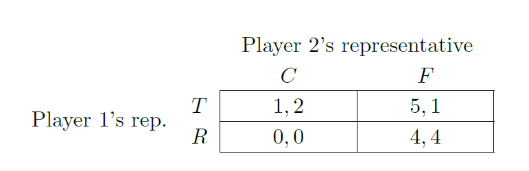
Proposition (Example) 7. Let $\Gamma=(A_1,A_2,u_1,u_2)$ be the game of Table 6. Under Assumption 1, $\Gamma^s=(\{R\},A_2,u_1,u_2)$ is a strict SPI on $\Gamma$.

Proof. First consider $\Gamma$. We can apply Assumption 1 to eliminate Player 1's $R_1$ and then apply Assumption 1 again to the resulting game to also eliminate Player 2's $R$. By transitivity, we find $\Gamma \sim_{\Phi} \Gamma'$, where $\Gamma'=(\{T\},\{C\},u_1,u_2)$ and $\Phi(T,C)=\{(T,C)\}$ and $\Phi(A_1\times A_2-\{(T,C)\})=\emptyset$.

Next, consider $\Gamma^s$. We can apply Assumption 1 to remove Player 2's strategy $C$ and find $\Gamma^s\sim_{\Psi} \hat \Gamma ^s$, where $\hat \Gamma ^s =(\{R\},\{F\},u_1,u_2)$ and $\Psi(R,F)=\{(R,F)\}$ and $\Psi(R,C)=\emptyset$.

Third, $\Gamma'\sim_{\mathrm{all}} \hat \Gamma^s$ by Lemma 2.5, where $\mathrm{all}(T,C)=\{(R,F)\}$.

Finally, we can apply transitivity to conclude $\Gamma \sim_{\Xi} \Gamma ^s$, where $\Xi= \Psi^{-1} \circ \mathrm{all} \circ \Phi$. It is easy to verify that $\Xi(T,C)=(R,F)$ and $\Xi(A_1\times A_2-\{(R,F)\})=\emptyset$. Hence, $\Xi$ is Pareto-improving and so by Theorem 3, $\Gamma^s$ is an SPI on $\Gamma$.

Note that in this example, Player 1 simply commits to a particular strategy $R$ and Player 2 maximizes their utility given Player 1's choice. Hence, this SPI can be justified with much simpler unilateral commitment setups [11, 52, 59]. For example, if the Temptation Game was played as a sequential game in which Player 1 plays first, its unique subgame-perfect equilibrium is $(R,F)$.

In Table 4 we give the Complicated Temptation Game, which better illustrates the features specific to our setup. Roughly, it is an extension of the simpler Temptation Game of Table 6. In addition to choosing $T$ versus $R$ and $C$ versus $F$, the players also have to make an additional choice (1 versus 2), which is difficult in that it cannot be solved by strict dominance. As we have argued in Section 3.1, the game in Table 5 is a unilateral SPI on Table 4. We can now show this formally.

Proposition (Example) 8. Let $\Gamma$ be the Complicated Temptation Game (Table 4) and $\Gamma^s$ be the subset game in Table 5. Under Assumptions 1 and 2, $\Gamma^s$ is a unilateral SPI on $\Gamma$.

Proof. In $\Gamma$, for Player 1, $T_1$ and $T_2$ strictly dominate $R_1$ and $R_2$. We can thus apply Assumption 1 to eliminate Player 1's $R1$ and $R_2$. In the resulting game, Player 2's $C_1$ and $C_2$ strictly dominate $F_1$ and $F_2$, so one can apply Assumption 1 again to the resulting game to also eliminate Player 2's $F_1$ and $F_2$. By transitivity, we find $\Gamma \sim_{\Phi} \Gamma'$, where $\Gamma'=(\{T_1,T_2\},\{C_1,C_2\},u_1,u_2)$ and

$$\begin{equation*} \Phi(a_1,a_2)=\left\{\begin{array}{cl} \{(a_1,a_2)\} & \text{if} \; a_1\in \{T_1,T_2\} \text{ and }a_2\in\{C_1,C_2\}\\ \emptyset & \text{otherwise}\\ \end{array}\right.. \end{equation*}$$

Next, consider $\Gamma^s$ (Table 5). We can apply Assumption 1 to remove Player 2's strategies $C_1$ and $C_2$ and find $\Gamma^s\sim_{\Psi} \hat \Gamma ^s$, where $\hat \Gamma ^s =(\{R_1,R_2\},\{F_1,F_2\},u_1^s,u_2)$ and

$$\begin{equation*} \Psi(a_1,a_2)=\left\{\begin{array}{cl} \{(a_1,a_2)\} & \text{if } a_1\in \{R_1,R_2\}\text{ and }a_2\in\{F_1,F_2 \}\\ \emptyset & \text{otherwise}\\ \end{array}\right.. \end{equation*}$$

Third, $\Gamma'\sim_{\Xi} \hat \Gamma^s$ by Assumption 2, where $\Xi$ decomposes into $\Xi_1$ and $\Xi_2$, corresponding to the two players, respectively, where $\Xi_1(T_i)=R_i$ and $\Xi_2(C_i)=F_i$ for $i=1,2$.

Finally, we can apply transitivity and the rule about symmetry and inverses (Lemma 2.2) to conclude $\Gamma \sim_{\Psi^{-1}\circ \Xi\circ \Phi} \Gamma ^s$. It is easy to verify that $\Psi^{-1}\circ \Xi\circ \Phi$ is Pareto-improving.

4.6 Computing safe Pareto improvements

In this section, we ask how computationally costly it is for the original players to identify for a given game $\Gamma$ a non-trivial SPI $\Gamma^s$. Of course, the answer to this question depends on what the original players are willing to assume about how their representatives act. For example, if only trivial outcome correspondences (as per Lemma 2.1 and 2.5) are assumed, then the decision problem is easy. Similarly, if $\Gamma\sim_{\Phi}\Gamma'$ for given $\Phi$ is hard to decide (e.g., because it requires solving for the Nash equilibria of $\Gamma$ and $\Gamma'$), then this could trivially also make the safe Pareto improvement problem hard to decide. We specifically are interested in deciding whether a given game $\Gamma$ has a non-trivial SPI that can be proved using only Assumptions 1 and 2, the general properties of game correspondence (in particular Transitivity (Lemma 2.3), Symmetry (Lemma 2.2) and Theorem 3).

Definition 5. The SPI decision problem consists in deciding for any given $\Gamma$, whether there is a game $\Gamma^s$ and a sequence of outcome correspondences $\Phi^1,...,\Phi^k$ and a sequence of subset games $\Gamma^0=\Gamma, \Gamma^1,...,\Gamma^k=\Gamma^s$ of $\Gamma$ s.t.:

1.  (Non-triviality:) If we fully reduce $\Gamma^s$ and $\Gamma$ using iterated strict dominance (Assumption 1), the two resulting games are not equal. (Of course, they are allowed to be isomorphic.)
2. For $i=1,...,k$, $\Gamma^{i-1}\sim_{\Phi^{i}} \Gamma^{i}$ is valid by a single application of either Assumption 1 or Assumption 1, or an application of Assumption 1 in reverse via Lemma 2.2. 
3. For all $\mathbf{a}\in A$, and whenever $\mathbf{a}^s\in (\Phi^k \circ \Phi ^{k-1} \circ ... \circ \Phi^{1})(\mathbf{a})$, it is the case that $u(\mathbf{a}^s) \geq \mathbf{u}(\mathbf{a})$.
   For the strict SPI decision problem, we further require:
4. There is a player $i$ and an outcome $\mathbf{a}$ that survives iterated elimination of strictly dominated strategies from $\Gamma$ s.t. $u_i((\Phi^k \circ \Phi ^{k-1} \circ ... \circ \Phi^{1})(\mathbf{a}))>u_i(\mathbf{a})$.
   For the unilateral SPI decision problem, we further require:
5. For all but one of the players $i$, $u_i=u_i^s$ and $A_i=A_i^s$.

Many variants of this problem may be considered. For example, to match Definition 1, the definition of the strict SPI problem assumes that all outcomes $\mathbf{a}$ that survive iterated elimination occur with positive probability. Alternatively we could have required that for demonstrating strictness, there must be a player $i$ such that for all $\mathbf{a}\in A$ that survive iterated elimination, $u_i((\Phi^k \circ \Phi ^{k-1} \circ ... \circ \Phi^{1})(\mathbf{a}))>u_i(\mathbf{a})$. Similarly one may wish to find SPIs that are strict improvements for all players. We may also wish to allow the use of the elimination of duplicate strategies (as described in Section 4.4.4) or trivial outcome correspondence steps as per Lemma 2.5. These modifications would not change the computational complexity of the problem, nor would they require new proof ideas. One may also wish to compute all SPIs, or – in line with multi-criteria optimization [14, 58] – all SPIs that cannot in turn be safely Pareto-improved upon. However, in general there may exist exponentially many such SPIs. To retain any hope of developing an efficient algorithm, one would therefore have to first develop a more efficient representation scheme [cf. 42, Sect. 16.4].

Theorem 9. The (strict) (unilateral) SPI decision problem is NP-complete, even for 2-player games.

Proposition 10. For games $\Gamma$ with $|A_1|+...+|A_n|=m$ that can be reduced (via iterative application of Assumption 1) to a game $\Gamma'$ with $|A_1'|+...+|A_n'|=l$, the (strict) (unilateral) SPI decision problem can be solved in $O(m^l)$.

The full proof is tedious (see Appendix D), but the main idea is simple, especially for omnilateral SPIs. To find an omnilateral SPI on $\Gamma$ based on Assumptions 1 and 2, one has to first iteratively remove all strictly dominated actions to obtain a reduced game $\Gamma'$, which the representatives would play the same as the original game. This can be done in polynomial time. One then has to map the actions $\Gamma'$ onto the original $\Gamma$ in such a way that each outcome in $\Gamma'$ is mapped onto a weakly Pareto-better outcome in $\Gamma$. Our proof of NP-hardness works by reducing from the subgraph isomorphism problem, where the payoff matrices of $\Gamma'$ and $\Gamma$ represent the adjacency matrices of the graphs.

Besides being about a specific set of assumptions about $\sim$, note that Theorem 9 and Proposition 10 also assume that the utility function of the game is represented explicitly in normal form as a payoff matrix. If we changed the game representation (e.g., to boolean circuits, extensive form game trees, quantified boolean formulas, or even Turing machines), this can affect the complexity of the SPI problem. For example, Gabarró, García, and Serna [16] show that the game isomorphism problem on normal-form games is equivalent to the graph isomorphism problem, while it is equivalent to the (likely computationally harder) boolean circuit isomorphism problem for a weighted boolean formula game representation. Solving the SPI problem requires solving a subset game isomorphism problem (see the proof of Lemma 28 in Appendix D for more detail). We therefore suspect that the SPI problem analogously increases in computational complexity (perhaps to being $\Sigma_2^p$-complete) if we treat games in a weighted boolean formula representation. In fact, even reducing a game using strict dominance by pure strategies – which contributes only insignificantly to the complexity of the SPI problem for normal-form games – is difficult in some game representations [10, Section 6]. Note, however, that for any game representation to which 2-player normal-form games can be efficiently reduced – such as, for example, extensive-form games – the hardness result also applies.

5 Safe Pareto improvements under improved coordination

5.1 Setup

In this section, we imagine that the players are able to simply invent new token strategies with new payoffs that arise from mixing existing feasible payoffs. To define this formally, we first define for any game $\Gamma=(A,\mathbf{u})$,

$$\begin{equation*} \mathcal{C}(\Gamma)\coloneqq \mathbf{u}(\Delta(A)) =\left\{ \sum_{\mathbf{a}\in A} p_{\mathbf{a}} {\mathbf{u}} (\mathbf{a}) \;\middle|\; \sum_{\mathbf{a}\in A} p_{\mathbf{a}} =1 \text{ and } \forall \mathbf{a}\in A\colon p_{\mathbf{a}}\in [0,1] \right\} \end{equation*}$$

to be the set of payoff vectors that are feasible by some correlated strategy. The underlying notion of correlated strategies is the same as in correlated equilibrium [2, 3], but in this paper it will not be relevant whether any such strategy is a correlated equilibrium of $\Gamma$. Instead their use will hinge on the use of commitments [cf. 34]. Note that $\mathcal{C}(\Gamma)$ is exactly the convex closure of $\mathbf{u}(A)$, i.e., the convex closure of the set of deterministically achievable utilities of the original game.

For any game $\Gamma$, we then imagine that in addition to subset games, the players can let the representatives play a perfect-coordination token game $(A^s,\mathbf{u}^s,\mathbf{u}^e)$, where for all $i$, $A_i^s\cap A_i=\emptyset$ and $u_i^s\colon A^s \rightarrow \mathbb{R}$ are arbitrary utility functions to be used by the representatives and ${\mathbf{u}}^e\colon A^s \rightarrow \mathcal{C}(\Gamma)$ are the utilities that the original players assign to the token strategies.

The instruction $(A^s,\mathbf{u}^s,\mathbf{u}^e)$ lets the representatives play the game $(A^s,\mathbf{u}^s)$ as usual. However, the strategies $A^s$ are imagined to be meaningless token strategies which do not resolve the given game $\Gamma$. Once some token strategies $\mathbf{a}^s$ are selected, these are translated into some probability distribution over $A$, i.e., into a correlated strategy of the original game. This correlated strategy is then played by the original players, thus giving rise to (expected) utilities ${\mathbf{u}}^e(\mathbf{a}^s)\in \mathcal{C}(\Gamma)$. These distributions and thus utilities are specified by the original players.

Definition 6. Let $\Gamma$ be a game. A perfect-coordination SPI for $\Gamma$ is a perfect-coordination token game $(A^s,\mathbf{u}^s,\mathbf{u}^e)$ for $\Gamma$ s.t. $\mathbf{u}^e(\Pi(A^s,u^s))\geq \mathbf{u} (\Pi(\Gamma))$ with certainty. We call $(A^s,\mathbf{u}^s,\mathbf{u}^e)$ a strict perfect-coordination SPI if there furthermore is a player $i$ for whom $u^e_i(\Pi(A^s,u^s))> u_i (\Pi(\Gamma))$ with positive probability.

As an example, imagine that $\Gamma$ is just the $\mathrm{DM}$-$\mathrm{RM}$ subset game of the Demand Game of Table 1. Then, intuitively, an SPI under improved coordination could consist of the original players telling the representatives, “Play as if you were playing the $\mathrm{DM}$-$\mathrm{RM}$ subset game of the Demand Game, but whenever you find yourself playing $(\mathrm{DM}, \mathrm{DM})$, randomize [according to some given distribution] between the other (Pareto-optimal) outcomes instead”. Formally, $A_1^s=\{\hat D,\hat R\}$ and $A_2^s=\{\hat D,\hat R\}$ would then consist of tokenized versions of the original strategies. The utility functions $u_1^s$ and $u_2^s$ are then simply the same as in the original Demand Game except that they are applied to the token strategies. For example, $\mathbf{u}^s(\hat D, \hat R)=(2,0)$. The utilities for the original players remove the conflict outcome. For example, the original players might specify ${\mathbf{u}}^e(\hat D,\hat D)=(1,1)$, representing that the representatives are supposed to play $(\mathrm{RM},\mathrm{RM})$ in the $(\hat D,\hat D)$ case. For all other outcomes $(\hat a_1,\hat a_2)$, it must be the case that ${\mathbf{u}}^e(\hat a_1,\hat a_2) ={\mathbf{u}}^s(\hat a_1,\hat a_2)$ because the other outcomes cannot be Pareto-improved upon. As with our earlier SPIs for the Demand Game, Assumption 2 implies that $\Gamma\sim_{\Phi} \Gamma^s$, where $\Phi$ maps the original conflict outcome $(\mathrm{DM}, \mathrm{DM})$ onto the Pareto-optimal ($\hat D$,$\hat D$).

Relative to the SPIs considered up until now, these new types of instructions put significant additional requirements on how the representatives interact. They now have to engage in a two-round process of first choosing and observing one another's token strategies and then playing a correlated strategy for the original game. Further, it must be the case that this additional coordination does not affect the payoffs of the original outcomes. The latter may not be the case in, e.g., the Game of Chicken. That is, we could imagine a Game of Chicken in which coordination is possible but that the rewards of the game change if the players do coordinate. After all, the underlying story in the Game of Chicken is that the positive reward – admiration from peers – is attained precisely for accepting a grave risk.

5.2 Finding safe Pareto improvement under improved representative coordination

With these more powerful ways to instruct representatives, we can now replace individual outcomes of the default game ad libitum. For example, in the reduced Demand Game, we singled out the outcome $(\mathrm{DM}, \mathrm{DM})$ as Pareto-suboptimal and replaced it by a Pareto-optimal outcome, while keeping all other outcomes the same. This allows us to construct SPIs in many more games than before.

Definition 7. The strict full-coordination SPI decision problem consists in deciding for any given $\Gamma$ whether under Assumption 2 there is a perfect-coordination SPI $\Gamma^s$ for $\Gamma$.

Lemma 11. For a given $n$-player game $\Gamma$ and payoff vector $\mathbf{y}\in \mathbb{R}^n$, it can be decided by linear programming and thus in polynomial time whether $\mathbf{y}$ is Pareto-optimal in $\mathcal{C}(\Gamma)$.

For an introduction to linear programming, see, e.g., Schrijver [50]. In short, a linear program is a specific type of constrained optimization problem that can be solved efficiently.

Proof. Finding a Pareto improvement on a given $\mathbf{y}\in \mathbb{R}^n$ can be formulated as the following linear program:

$$\begin{align*} \text{Variables:}\quad & p_{\mathbf{a}}\in [0,1] \textup{ for all }\mathbf{a}\in A\\ \textup{Maximize}\quad & \sum_{i=1}^n \left(\sum_{\mathbf{a}\in A} p_{\mathbf{a}} u_i(\mathbf{a}) \right) - y_i \\ \textup{s.t.}\quad & \sum_{\mathbf{a}\in A} p_{\mathbf{a}}=1\\ & \sum_{\mathbf{a}\in A} p_{\mathbf{a}} u_i(\mathbf{a}) \geq y_i \textup{ for }i=1,...,n \end{align*}$$

Based on Lemma 11, Algorithm 1 decides whether there is a strict perfect-coordination SPI for a given game $\Gamma$.

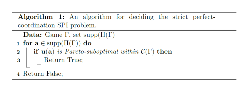
It is easy to see that this algorithm runs in polynomial time (in the size of, e.g., the normal form representation of the game). It is also correct: if it returns True, simply replace the Pareto-suboptimal outcome while keeping all other outcomes the same; if it returns False, then all outcomes are Pareto-optimal within $\mathcal{C}(\Gamma)$ and so there can be no strict SPI. We summarize this result in the following proposition.

Proposition 12. Assuming $\mathrm{supp}(\Pi(\Gamma))$ is known and that Assumption 2 holds, it can be decided in polynomial time whether there is a strict perfect-coordination SPI.

5.3 Characterizing safe Pareto improvements under improved representative coordination

From the problem of deciding whether there are strict SPIs under improved coordination at all, we move on to the question of what different perfect-coordination SPIs there are. In particular, one might ask what the cost is of only considering safe Pareto improvements relative to acting on a probability distribution over $\Pi(\Gamma)$ and the resulting expected utilities $\mathbb{E}\left[\mathbf{u}(\Pi(\Gamma))\right]$. We start with a lemma that directly provides a characterization. So far, all the considered perfect-coordination SPIs $(A^s,\mathbf{u}^s,\mathbf{u}^e)$ for a game $(A,\mathbf{u})$ have consisted in letting the representatives play a game $(A^s,\mathbf{u}^s)$ that is isomorphic to the original game, but Pareto-improves (from the original players' perspectives, i.e., $\mathbf{u}^e$) at least one of the outcomes. It turns out that we can restrict attention to this very simple type of SPI under improved coordination.

Lemma 13. Let $\Gamma=(\{a_1^1,...,a_1^{l_1}\},...,\{a_n^1,...,a_n^{l_n}\},\mathbf{u})$ be any game. Let $\Gamma'$ be a perfect-coordination SPI on $\Gamma$. Then we can define ${\mathbf{u}}^e$ with values in $\mathcal{C}(\Gamma)$ such that under Assumption 2 the game

$$\begin{equation*}\begin{split}\Gamma^s=\bigg(& \hat A_1\coloneqq \{\hat a_1^1,...,\hat a_1^{l_1}\},...,\hat A_n\coloneqq\{\hat a_n^1,...,\hat a_n^{l_n}\},\\&~~~\hat{ \mathbf{u}}\colon (\hat a_1^{i_1},...,\hat a_n^{i_n})\mapsto \mathbf{u}( a_1^{i_1},..., a_n^{i_n}),\mathbf{u}^e \bigg)\end{split}\end{equation*}$$

is also an SPI on $\Gamma$, with

$$\mathbb{E}\left[ {\mathbf{u}}(\Pi(\Gamma^s)) \;\middle|\; \Pi(\Gamma){=}\mathbf{a} \right] = \mathbb{E}\left[ {\mathbf{u}}(\Pi(\Gamma^\prime)) \;\middle|\; \Pi(\Gamma){=}\mathbf{a} \right]$$

for all $\mathbf{a}\in A$ and consequently $\mathbb{E}\left[ {\mathbf{u}}(\Pi(\Gamma^s)) \right] = \mathbb{E}\left[ {\mathbf{u}}(\Pi(\Gamma')) \right]$.

Proof. First note that $(\hat A,\hat{\mathbf{u}})$ is isomorphic to $\Gamma$. Thus by Assumption 2, there is isomorphism $\Phi$ s.t. $\Gamma \sim_{\Phi} (\hat A,\hat{\mathbf{u}})$. WLOG assume that $\Phi$ simply maps $a_1^{i_1},..., a_n^{i_n} \mapsto \hat a_1^{i_1},...,\hat a_n^{i_n}$. Then define $\mathbf{u}^e$ as follows:

$$\begin{equation*} \mathbf{u}^e(\hat a_1^{i_1},...,\hat a_n^{i_n})=\mathbb{E}\left[ {\mathbf{u}}' (\Pi(\Gamma')) \mid \Pi(\Gamma)=( a_1^{i_1},...,a_n^{i_n}) \right]. \end{equation*}$$

Here ${\mathbf{u}}'$ describes the utilities that the original players assign to the outcomes of $\Gamma'$. Since ${\mathbf{u}}'$ maps onto $\mathcal{C}(\Gamma)$ and $\mathcal{C}(\Gamma)$ is convex, $\mathbf{u}^e$ as defined also maps into $\mathcal{C}(\Gamma)$ as required. Note that for all $a_1^{i_1},...,a_n^{i_n}$ it is by assumption ${\mathbf{u}}' (\Pi(\Gamma'))\geq {\mathbf{u}}(a_1^{i_1},...,a_n^{i_n})$ with certainty. Hence,

$$\begin{aligned} u^e(\hat a_1^{i_1},...,\hat a_n^{i_n}))&= \mathbb{E}\left[ \mathbf{u}' (\Pi(\Gamma')) \mid \Pi(\Gamma)=( a_1^{i_1},...,a_n^{i_n}) \right]\\ &\geq {\mathbf{u}}( a_1^{i_1},...,a_n^{i_n}), \end{aligned}$$

as required.

Because of this result, we will focus on these particular types of SPIs, which simply create an isomorphic game with different (Pareto-better) utilities. Note, however, that without assigning exact probabilities to the distributions of $\Pi(\Gamma),\Pi(\Gamma')$, the original players will in general not be able to construct a $\Gamma^s$ that satisfies the expected payoff equalities. For this reason, one could still conceive of situations in which a different type of SPI would be chosen by the original players and the original players are unable to instead choose an SPI of the type described in Lemma 13.

Lemma 13 directly implies a characterization of the expected utilities that can be achieved with perfect-coordination SPIs. Of course, this characterization depends on the exact distribution of $\Pi(\Gamma)$. We omit the statement of this result. However, we state the following implication.

Corollary 14. Under Assumption 2, the set of Pareto improvements that are safely achievable with perfect coordination

$$\begin{equation*}\{ \mathbb{E}[ {\mathbf{u}}(\Gamma') ]\mid \Gamma'\text{ is perfect-coordination SPI on }\Gamma \}\end{equation*}$$

is a convex polygon.

Because of this result, one can also efficiently optimize convex functions over the set of perfect-coordination SPIs. Even without referring to the distribution $\Pi(\Gamma)$, many interesting questions can be answered efficiently. For example, we can efficiently identify the perfect-coordination SPI that maximizes the minimum improvements across players and outcomes $\mathbf{a}\in A$.

In the following, we aim to use Lemma 13 and Corollary 14 to give maximally strong positive results about what Pareto improvements can be safely achieved, without referring to exact probabilities over $\Pi(\Gamma)$. To keep things simple, we will do this only for the case of two players. To state our results, we first need some notation: We use

$$\begin{equation*} \mathrm{PF}(\mathcal{C}) \coloneqq \left\{ \mathbf{y}\in \mathcal{C} \;\middle|\; \not\exists \mathbf{y}'{\in}\mathcal{C},i\in\{1,...,n\}: \mathbf{y}'\geq \mathbf{y}, y'_i>y \right\} \end{equation*}$$

to denote the Pareto frontier of a convex polygon $\mathcal{C}$ (or more generally convex, closed set). For any real number $x\in \mathbb{R}$, we use $\pi_i(x,\mathcal{C}(\Gamma))$ to denote the ${\mathbf{y}}'\in \mathcal{C}(\Gamma)$ which maximizes $y'_{-i}$ under the constraint $y'_{i}= x.$ (Recall that we consider 2-player games, so $y'_{-i}$ is a single real number.) Note that such a ${\mathbf{y}}'$ exists if and only if $x$ is $i$'s utility in some feasible payoff vector. We first state our result formally. Afterwards, we will give a graphical explanation of the result, which we believe is easier to understand.

Theorem 15. Make Assumption 2. Let $\Gamma$ be a two-player game. Let ${\mathbf{y}}\in \mathbb{R}^2$ be some potentially unsafe Pareto improvement on $\mathbb{E}\left[{\mathbf{u}}(\Pi(\Gamma)) \right]$. For $i=1,2$, let $x^{\mathrm{min}/\mathrm{max}}_i=\min/\max u_i\left( \mathrm{supp}(\Pi(\Gamma)) \right)$. Then:

A) If there is some element in $\mathcal{C}(\Gamma)$ which Pareto-dominates all of $\mathrm{supp}(\Pi(\Gamma))$ and if ${\mathbf{y}}$ is Pareto-dominated by an element of at least one of the following three sets:

•  $L_1\coloneqq$ the line segment between $\pi_1(x_1^{\mathrm{min}},\mathrm{PF}(\mathcal{C}(\Gamma))$ and $\pi_1(x_1^{\mathrm{max}},\mathrm{PF}(\mathcal{C}(\Gamma))$;
• $L_2\coloneqq$ the segment of the curve $\mathrm{PF}(\mathcal{C}(\Gamma))$ between $\pi_{1}(x^{\mathrm{max}}_1 , \mathrm{PF}(\mathcal{C}(\Gamma))))$ and $\pi_{2}(x^{\mathrm{max}}_2, \mathrm{PF}(\mathcal{C}(\Gamma))))$;
• $L_3\coloneqq$ the line segment between $\pi_2(x_2^{\mathrm{max}},\mathrm{PF}(\mathcal{C}(\Gamma))$ and $\pi_2(x_2^{\mathrm{min}},\mathrm{PF}(\mathcal{C}(\Gamma))$.

Then there is an SPI under improved coordination $\Gamma^s$ such that $\mathbb{E}\left[{\mathbf{u}}(\Pi(\Gamma^s)) \right]={\mathbf{y}}$.

B) If there is no element in $\mathcal{C}(\Gamma)$ which Pareto-dominates all of $\mathrm{supp}(\Pi(\Gamma))$ and if $\mathbf{y}$ is Pareto-dominated by an element each of $L_1$ and $L_3$ as defined above, then there is a perfect-coordination SPI $\Gamma^s$ such that $\mathbb{E}\left[{\mathbf{u}}(\Pi(\Gamma^s)) \right]={\mathbf{y}}$.

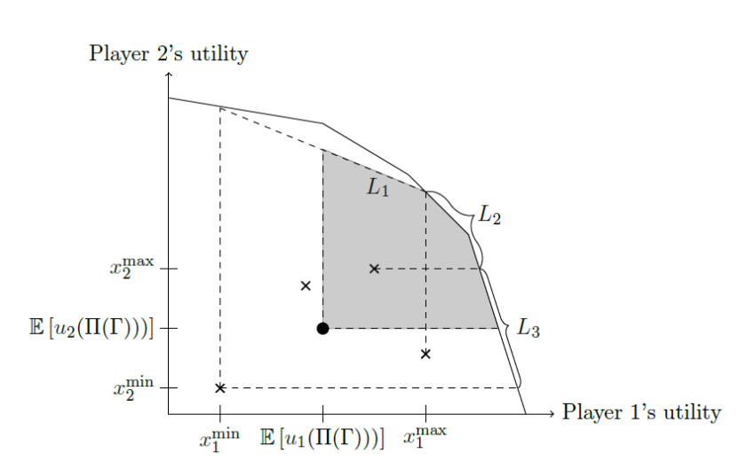
We now illustrate the result graphically. We start with Case A, which is illustrated in Figure 2. The Pareto-frontier is the solid line in the north and east. The points marked x indicate outcomes in $\mathrm{supp}(\Pi(\Gamma))$. The point marked by a filled circle indicates the expected value of the default equilibrium $\mathbb{E}\left[ {\mathbf{u}} (\Pi(\Gamma)) \right]$. The vertical dashed lines starting at the two extreme x marks illustrate the application of $\pi_1$ to project $x_1^{\mathrm{min}/\mathrm{max}}$ onto the Pareto frontier. The dotted line between these two points is $L_1$. Similarly, the horizontal dashed lines starting at x marks illustrate the application of $\pi_2$ to project $x_2^{\mathrm{min}/\mathrm{max}}$ onto the Pareto frontier. The line segment between these two points is $L_3$. In this case, this line segments lies on the Pareto frontier. The set $L_2$ is simply that part of the Pareto frontier, which Pareto-dominates all elements of $\mathrm{supp}(\Pi(\Gamma))$, i.e., the part of the Pareto frontier to the north-east between the two intersections with the northern horizontal dashed line and eastern vertical dashed line. The theorem states that for some ${\mathbf{y}}\in \mathbb{R}^2$ to be a Pareto improvement, it must be in the gray area.

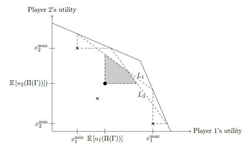
Case B of Theorem 15 is depicted in Figure 3. Note that here the two line segments $L_1$ and $L_3$ intersect. To ensure that a Pareto improvement is safely achievable, the theorem requires that it is below both of these lines, as indicated again by the gray area.

 

For a full proof, see Appendix E. Roughly, Theorem 15 is proven by re-mapping each of the outcomes of the original game as per Lemma 13. For example, the projection of the default equilibrium $\mathbb{E}\left[\mathbf{u}(\Pi(\Gamma))\right]$ (i.e., the filled circle) onto $L_1$ is obtained as an SPI by projecting all the outcomes (i.e., all the x marks) onto $L_1$. In Case A, any utility vector $\mathbf{y}\in L_2$ that Pareto-improves on all outcomes of the original game can be obtained by re-mapping all outcomes onto $\mathbf{y}$. Other kinds of $\mathbf{y}$ are handled similarly.

As a corollary of Theorem 15, we can see that all (potentially unsafe) Pareto improvements in the $\mathrm{DM}$-$\mathrm{RM}$ subset game of the Demand Game of Table 1 are equivalent to some perfect-coordination SPI. However, this is not always the case:

Proposition 16. There is a game $\Gamma=(A,\mathbf{u})$, representatives $\Pi$ that satisfy Assumptions 1 and 2, and an outcome $\mathbf{a}\in A$ s.t. $u_i(\mathbf{a})>\mathbb{E}\left[ u_i(\Pi(\Gamma)) \right]$ for all players $i$, but there is no perfect-coordination SPI $(A^s,\mathbf{u}^s,\mathbf{u}^e)$ s.t. for all players $i$, $\mathbb{E}\left[ u^e_i(\Pi(A^s,\mathbf{u}^s)) \right] = u_i(\mathbf{a})$.

As an example of such a game, consider the game in Table 7. Strategy $c$ can be eliminated by strict dominance (Assumption 1) for both players, leaving a typical Chicken-like payoff structure with two pure Nash equilibria ($(a,b)$ and $(b,a)$), as well as a mixed Nash equilibrium $(3/8*a+5/8*b,3/8*a+5/8*b)$.

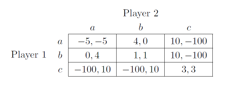
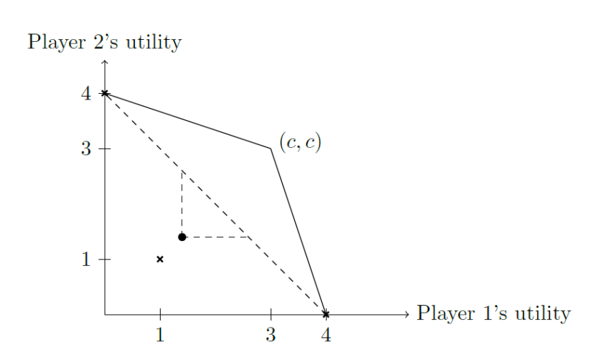
Now let us say that in the resulting game $P(\Pi(\Gamma){=}(a,b))=p=P(\Pi(\Gamma){=}(b,a))$ for some $p$ with $0< p \leq \nicefrac{1}{2}$. Then one (unsafe) Pareto improvement would be to simply always have the representatives play $(c,c)$ for a certain payoff of $(3,3)$. Unfortunately, there is no safe Pareto improvement with the same expected payoff. Notice that $(3,3)$ is the unique element of $\mathcal{C}(\Gamma)$ that maximizes the sum of the two players' utilities. By linearity of expectation and convexity of $\mathcal{C}(\Gamma)$, if for any $\Gamma ^s$ it is $\mathbb{E}\left[{\mathbf{u}}(\Pi(\Gamma ^s)) \right]=(3,3)$, it must be ${\mathbf{u}}(\Pi(\Gamma ^s))=(3,3)$ with certainty. Unfortunately, in any safe Pareto improvement the outcomes $(a,b)$ and $(b,a)$ must corresponds to outcomes that still gives utilities of $(4,0)$ and $(0,4)$, respectively, because these are Pareto-optimal within the set of feasible payoff vectors. We illustrate this as an example of Case B of Theorem 15 in Figure 4.

6 The SPI selection problem

In the Demand Game, there happens to be a single non-trivial SPI. However, in general (even without the type of coordination assumed in Section 5) there may be multiple SPIs that result in different payoffs for the players. For example, imagine an extension of the Demand Game imagine that both players have an additional action $\mathrm{DL}'$, which is like $\mathrm{DL}$, except that under $(\mathrm{DL}', \mathrm{DL}')$, Aliceland can peacefully annex the desert. Aliceland prefers this SPI over the original one, while Bobbesia has the opposite preference. In other cases, it may be unclear to some or all of the players which of two SPIs they prefer. For example, imagine a version of the Demand Game in which one SPI mostly improves on $(\mathrm{DM},\mathrm{DM})$ and another mostly improves on the other three outcomes, then outcome probabilities are required for comparing the two. If multiple SPIs are available, the original players would be left with the difficult decision of which SPI to demand in their instruction.⁹

This difficulty of choosing what SPI to demand cannot be denied. However, we would here like to emphasize that players can profit from the use of SPIs even without addressing this SPI selection problem. To do so, a player picks an instruction that is very compliant (“dove-ish”) w.r.t. what SPI is chosen, e.g., one that simply goes with whatever SPI the other players demand as long as that SPI cannot further be safely Pareto-improved upon.¹⁰ In many cases, all such SPIs benefit all players. For example, optimal SPIs in bargaining scenarios like the Demand Game remove the conflict outcome, which benefits all parties. Thus, a player can expect a safe improvement even under such maximally compliant demands on the selected SPI.

In some cases there may also be natural choices of demands (a là Schelling [48, pp. 54–58] or focal points). If the underlying game is symmetric, a symmetric safe Pareto improvement may be a natural choice. For example, the fully reduced version of the Demand Game of Table 1 is symmetric. Hence, we might expect that even if multiple SPIs were available, the original players would choose a symmetric one.

7 Conclusion and future directions

Safe Pareto improvements are a promising new idea for delegating strategic decision making. To conclude this paper, we discuss some ideas for further research on SPIs.

Straightforward technical questions arise in the context of the complexity results of Section 4.6. First, what impact on the complexity does varying the assumptions have? Our NP-completeness proof is easy to generalize at least to some other types of assumptions. It would be interesting to give a generic version of the result. We also wonder whether there are plausible assumptions under which the complexity changes in interesting ways. Second, one could ask how the complexity changes if we use more sophisticated game representations (see the remarks at the end of that section). Third, one could impose additional restrictions on the sought SPI. Fourth, we could restrict the games under consideration. Are there games in which it becomes easy to decide whether there is an SPI?

It would also be interesting to see what real-world situations can already be interpreted as utilizing SPIs, or could be Pareto-improved upon using SPIs.

Acknowledgments

This work was supported by the National Science Foundation under Award IIS-1814056. Some early work on this topic was conducted by Caspar Oesterheld while working at the Foundational Research Institute (now the Center on Long-Term Risk). For valuable comments and discussions, we are grateful to Keerti Anand, Tobias Baumann, Jesse Clifton, Max Daniel, Lukas Gloor, Adrian Hutter, Vojtěch Kovařík, Anni Leskelä, Brian Tomasik and Johannes Treutlein, and our wonderful anonymous referees. We also thank attendees of a 2017 talk at the Future of Humanity Institute at the University of Oxford, a talk at the May 2019 Effective Altruism Foundation research retreat, and our talk at AAMAS 2021.

References

[1] Krzysztof R. Apt. “Uniform Proofs of Order Independence for Various Strategy Elimination Procedures”. In: The B.E. Journal of Theoretical Economics 4.1 (2004), pp. 1–48. DOI: 10.2202/1534-5971.1141.

[2] Robert J. Aumann. “Correlated Equilibrium as an Expression of Bayesian Rationality”. In: Econometrica 55.1 (Jan. 1987), pp. 1–18. DOI: 10.2307/1911154.

[3] Robert J. Aumann. “Subjectivity and Correlation in Randomized Strategies”. In: Journal of Mathematical Economics 1.1 (Mar. 1974), pp. 67–97. DOI: 10.1016/0304-4068(74)90037-8.

[4] Robert Axelrod. The Evolution of Cooperation. New York: Basic Books, 1984.

[5] Mihaly Barasz et al. Robust Cooperation in the Prisoner’s Dilemma: Program Equilibrium via Provability Logic. Jan. 2014. url: https://arxiv.org/abs/1401.5577.

[6] Ken Binmore. Game Theory – A Very Short Introduction. Oxford University Press, 2007.

[7] Tilman Börgers. “Pure Strategy Dominance”. In: Econometrica 61.2 (Mar. 1993), pp. 423–430.

[8] Vitalik Buterin. Ethereum White Paper – A Next Generation Smart Contract & Decentralized Application Platform. Updated version available at https://github.com/ethereum/wiki/wiki/White-Paper. 2014. URL: https : //cryptorating . eu / whitepapers / Ethereum /Ethereum_white_paper.pdf.

[9] Andrew M. Colman. “Salience and focusing in pure coordination games”. In: Journal of Economic Methodology 4.1 (1997), pp. 61–81. DOI: 10.1080/13501789700000004.

[10] Vincent Conitzer and Tuomas Sandholm. “Complexity of (Iterated) Dominance”. In: Proceedings of the 6th ACM conference on Electronic commerce. Vancouver, Canada: Association for Computing Machinery, June 2005, pp. 88–97. DOI: 10.1145/1064009.1064019.

[11] Vincent Conitzer and Tuomas Sandholm. “Computing the Optimal Strategy to Commit to”. In: Proceedings of the ACM Conference on Electronic Commerce (EC). Ann Arbor, MI, USA: Association for Computing Machinery, 2006, pp. 82–90.

[12] Stephen A. Cook. “The complexity of theorem-proving procedures”. In: STOC ’71: Proceedings of the third annual ACM symposium on Theory of computing. New York: Association for Computing Machinery, May 1971, pp. 151–158. DOI: 10.1145/800157.805047.

[13] Andrew Critch. “A Parametric, Resource-Bounded Generalization of Löb’s Theorem, and a Robust Cooperation Criterion for Open-Source Game Theory”. In: Journal of Symbolic Logic 84.4 (Dec. 2019), pp. 1368–1381. DOI: 10.1017/jsl.2017.42.

[14] Matthias Ehrgott. Multicriteria Optimization. 2nd ed. Berlin: Springer, 2005.

[15] Lance Fortnow. “Program equilibria and discounted computation time”. In: Proceedings of the 12th Conference on Theoretical Aspects of Rationality and Knowledge (TARK ’09). July 2009, pp. 128–133. DOI: 10.1145/1562814.1562833.

[16] Joaquim Gabarró, Alina García, and Maria Serna. “The complexity of game isomorphism”. In: Theoretical Computer Science 412.48 (Nov. 2011), pp. 6675–6695. DOI:  10.1016/j.tcs.2011.07.022.

[17] David Gale. “A Theory of N-Person Games with Perfect Information”. In: Proceedings of the National Academy of Sciences of the United States of America 39.6 (June 1953), pp. 496–501. DOI: 10.1073/pnas.39.6.496.

[18] David Gauthier. “Coordination”. In: Dialogue 14.2 (June 1975), pp. 195–221. DOI: 10.1017/S0012217300043365.

[19] Itzhak Gilboa, Ehud Kalai, and Eitan Zemel. “On the order of eliminating dominated strategies”. In: Operations Research Letters 9.2 (Mar. 1990), pp. 85–89. DOI: 10.1016/0167-6377(90)90046-8.

[20] John C. Harsanyi and Reinhard Selten. A General Theory of Equilibrium Selection in Games. Cambridge, MA: The MIT Press, 1988.

[21] Bengt Robert Holmstr¨om. “On Incentives and Control in Organizations”. PhD thesis. Stanford University, Dec. 1977.

[22] J. V. Howard. “Cooperation in the Prisoner’s Dilemma”. In: Theory and Decision 24 (May 1988), pp. 203–213. DOI: 10.1007/BF00148954.

[23] Leonid Hurwicz and Leonard Shapiro. In: The Bell Journal of Economics 9.1 (1978), pp. 180–191. DOI: 10.2307/3003619.

[24] Adam Tauman Kalai et al. “A commitment folk theorem”. In: Games and Economic Behavior 69 (2010), pp. 127–137. DOI: 10.1016/j.geb.2009.09.008.

[25] Jon Kleinberg and Robert Kleinberg. “Delegated Search Approximates Efficient Search”. In: Proceedings of the 19th ACM Conference on Economics and Computation (EC). 2018.

[26] Frank H. Knight. Risk, Uncertainty, and Profit. Boston, MA, USA: Houghton Mifflin Company, 1921.

[27] Elon Kohlberg and Jean-Francois Mertens. “On the Strategic Stability of Equilibria”. In: Econometrica 54.5 (Sept. 1986), pp. 1003–1037. DOI: 10.2307/1912320.

[28] Jean-Jacques Laffont and David Martimort. The Theory of Incentives – The Principal-Agent Model. Princeton, NJ: Princeton University Press, 2002.

[29] Richard A. Lambert. “Executive Effort and Selection of Risky Projects”. In: RAND J. Econ. 17.1 (1986), pp. 77–88.

[30] David Lewis. Convention. Harvard University Press, 1969.

[31] R. Duncan Luce and Howard Raiffa. Games and Decisions. Introduction and Critical Survey. New York: Dover Publications, 1957.

[32] Leslie M. Marx and Jeroen M. Swinkels. “Order Independence for Iterated Weak Dominance”. In: Games and Economic Behavior 18 (1997), pp. 219–245. DOI: 10.1006/game.1997.0525.

[33] R. Preston McAfee. “Effective Computability in Economic Decisions”. May 1984. URL: https://www.mcafee.cc/Papers/PDF/EffectiveComputability.pdf.

[34] Dov Monderer and Moshe Tennenholtz. “Strong mediated equilibrium”. In: Artificial Intelligence 173.1 (Jan. 2009), pp. 180–195. DOI: 10.1016/j.artint.2008.10.005.

[35] John von Neumann. “Zur Theorie der Gesellschaftsspiele”. In: Mathematische Annalen 100 (1928), pp. 295–320. DOI: https://doi.org/10.1007/BF01448847.

[36] Caspar Oesterheld. “Robust Program Equilibrium”. In: Theory and Decision 86.1 (Feb. 2019), pp. 143–159.

[37] Caspar Oesterheld and Vincent Conitzer. “Minimum-regret contracts for principal-expert problems”. In: Proceedings of the 16th Conference on Web and Internet Economics (WINE). 2020.

[38] Hessel Oosterbeek, Randolph Sloof, and Gijs van de Kuilen. “Cultural Differences in Ultimatum Game Experiments: Evidence from a Meta-Analysis”. In: Experimental Economics 7 (June 2004), pp. 171–188. DOI: 10.1023/B:EXEC.0000026978.14316.74.

[39] Martin J. Osborne. An Introduction to Game Theory. New York: Oxford University Press, 2004.

[40] Martin J. Osborne and Ariel Rubinstein. A Course in Game Theory. The MIT Press, 1994.

[41] David G. Pearce. “Rationalizable Strategic Behavior and the Problem of Perfection”. In: Econometrica 54.4 (July 1984), pp. 1029–1050.

[42] Guillaume Perez. “Decision diagrams: constraints and algorithms”. PhD thesis. Université Côte d’Azur, 2017. URL: https : / / tel .archives-ouvertes.fr/tel-01677857/document.

[43] Martin Peterson. An Introduction to Decision Theory. Cambridge University Press, 2009.

[44] Steven Pinker. How the Mind Works. W. W. Norton, 1997.

[45] Werner Raub. “A General Game-Theoretic Model of Preference Adaptions in Problematic Social Situations”. In: Rationality and Society 2.1 (Jan. 1990), pp. 67–93.

[46] Ariel Rubinstein. Modeling Bounded Rationality. Ed. by Karl Gunnar Persson. Zeuthen Lecture Book Series. The MIT Press, 1998.

[47] Alexander Savelyev. “Contract law 2.0: ‘Smart’ contracts as the beginning of the end of classic contract law”. In: Information & Communications Technology Law 26.2 (2017), pp. 116–134. DOI: 10.1080/13600834.2017.1301036.

[48] Thomas C. Schelling. The Strategy of Conflict. Cambridge, MA: Harvard University Press, 1960.

[49] Thomas C. Schelling. “The Strategy of Conflict Prospectus for a Reorientation of Game Theory”. In: The Journal of Conflict Resolution 2.3 (Sept. 1958), pp. 203–264.

[50] Alexander Schrijver. Theory of Linear and Integer Programming. Chichester, UK: John Wiley & Sons, 1998.

[51] Amartya Sen. “Choice, orderings and morality”. In: Practical Reason. Ed. by Stephan Körner. New Haven, CT, USA: Basil Blackwell, 1974. Chap. II, pp. 54–67.

[52] Heinrich von Stackelberg. “Marktform und Gleichgewicht”. In: Vienna: Springer, 1934, pp. 58–70.

[53] Neal M. Stoughton. “Moral Hazard and the Portfolio Management Problem”. In: The Journal of Finance 48.5 (Dec. 1993), pp. 2009–2028. DOI: 10.1111/j.1540-6261.1993.tb05140.x.

[54] Robert Sugden. In: The Economic Journal 105.430 (May 1995), pp. 533–550. DOI: 10.2307/2235016.

[55] Moshe Tennenholtz. “Program equilibrium”. In: Games and Economic Behavior 49.2 (Nov. 2004), pp. 363–373.

[56] Johannes Treutlein et al. “A New Formalism, Method and Open Issues for Zero-Shot Coordination”. In: Proceedings of the Thirty-eighth International Conference on Machine Learning (ICML’21). 2021.

[57] Wiebe van der Hoek, Cees Witteveen, and Micheal Wooldridge. “Program equilibrium – a program reasoning approach”. In: International Journal of Game Theory 42 (3 Aug. 2013), pp. 639–671.

[58] Luc N. van Wassenhove and Ludo F. Gelders. “Solving a bicriterion scheduling problem”. In: European Journal of Operational Research 4 (1980), pp. 42–48.

[59] Bernhard Von Stengel and Shmuel Zamir. Leadership with commitment to mixed strategies. Tech. rep. LSE-CDAM-2004-01. London School of Economics, 2004. URL: http://www.cdam.lse.ac.uk/Reports/Files/cdam-2004-01.pdf.

---

A Proof of Theorem 1 – program equilibrium implementations of safe Pareto improvements

This paper considers the meta-game of delegation. SPIs are a proposed way of playing these games. However, throughout most of this paper, we do not analyze the meta-game directly as a game using the typical tools of game theory. We here fill that gap and in particular prove Theorem 1, which shows that SPIs are played in Nash equilibria of the meta game, assuming sufficiently strong contracting abilities. As noted, this result is essential. However, since it is mostly an application of existing ideas from the literature on program equilibrium, we left a detailed treatment out of the main text.

A program game for $\Gamma=(A,\mathbf{u})$ is defined via a set $\mathrm{PROG}=\mathrm{PROG}_1\times ... \times \mathrm{PROG}_n$ and a non-deterministic mapping $\mathit{exec}\colon \mathrm{PROG}_1\times ... \times \mathrm{PROG}_n \rightsquigarrow A$. We obtain a new game with action sets $\mathrm{PROG}$ and utility function

$$\begin{equation*} U\colon \mathrm{PROG}\rightarrow \mathbb{R}^n\colon \mathbf{c} \mapsto \mathbb{E}\left[ \mathbf{u}(\mathit{exec}(\mathbf{c})) \right]. \end{equation*}$$

Though this definition is generic, one generally imagines in the program equilibrium literature that for all $i$, $\mathrm{PROG}_i$ consists of computer programs in some programming language, such as Lisp, that take as input vectors in $\mathrm{PROG}$ and return an action $a_i$. The function $\mathit{exec}$ on input $\mathbf{c}\in \mathrm{PROG}$ then executes each player $i$'s program $c_i$ on $\mathbf{c}$ to assign $i$ an action. The definition implicitly assumes that $\mathrm{PROG}$ only contains programs that halt when fed one another as input (or that not halting is mapped onto some action). As is usually done in the program equilibrium literature, we will leave unspecified what constraints are used to ensure this. A program equilibrium is then simply a Nash equilibrium of the program game.

For the present paper, we add the following feature to the underlying programming language. A program can call a “black box subroutine” $\Pi_i(\Gamma')$ for any subset game $\Gamma'$ of $\Gamma$, where $\Pi_i(\Gamma')$ is a random variable over $A_i'$ and $\Pi(\Gamma')=(\Pi_1(\Gamma'),...,\Pi_n(\Gamma'))$.

We need one more definition. For any game $\Gamma$ and player $i$, we define Player $i$'s threat point (a.k.a. minimax utility) $v_i^{\Gamma}$ as

$$\begin{equation*} v_i^{\Gamma}=\min_{\boldsymbol{\sigma}_{-i} \in \bigtimes_{j\neq i} \Delta(A_{j})} ~ \max_{\sigma_i \in \Delta(A_i)} u_i (\sigma_i,\boldsymbol{\sigma}_{-i}). \end{equation*}$$

In words, $v_i^{\Gamma}$ is the minimum utility that the players other than $i$ can force onto $i$, under the assumption that $i$ reacts optimally to their strategy. We further will use $\mathit{minimax}(i,j)\in \Delta(A_j)$ to denote the strategy for Player $j$ that is played in the minimizer $\sigma_{-i}$ of the above. Of course, in general, there might be multiple minimizers $\sigma_{-i}$. In the following, we will assume that the function $\mathit{minimax}$ breaks such ties in some consistent way, such that for all $i$,

$$\begin{equation*} (\mathit{minimax}(i,j))_{j\in \{1,...,n\}-\{i\}} \in \argmin_{\boldsymbol{\sigma}_{-i} \in \bigtimes_{j\neq i} \Delta(A_{j})} ~ \max_{\sigma_i \in \Delta(A_i)} u_i (\sigma_i,\boldsymbol{\sigma}_{-i}). \end{equation*}$$

Note that for $n=2$, each player's threat point is computable in polynomial time via linear programming; and that by the minimax theorem [35], the threat point is equal to the maximin utility, i.e.,

$$\begin{equation*} v_i^{\Gamma}=\max_{\sigma_i \in \Delta(A_i)}~\min_{\sigma_{-i} \in \Delta(A_{-i})} u_i (\sigma_i,\sigma_{-i}), \end{equation*}$$

so $v_i^{\Gamma}$ is also the minimum utility that Player $i$ can guarantee for herself under the assumption that the opponent sees her mixed strategy and reacts in order to minimize Player $i$'s utility.

Tennenholtz’ [55] main result on program games is the following:

Theorem 17 (Tennenholtz 2004 [55]). Let $\Gamma=(A,\mathbf{u})$ be a game and let $\mathbf{x}\in \mathbf{u}\left(\bigtimes_{i=1}^n \Delta(A_i) \right)$ be a (feasible) payoff vector. If $x_i\geq v_i^{\Gamma}$ for $i=1,...,n$, then $\mathbf{x}$ is the utility of some program equilibrium of a program game on $\Gamma.$

Throughout the rest of this section, our goal is to use similar ideas as Tennenholtz did for Theorem 17 to construct for any SPI $\Gamma^s$ on $\Gamma$, a program equilibrium that results in the play of $\Pi(\Gamma^s)$. As noted in the main text, the Player $i$'s instruction to her representative to play the game $\Gamma ^s$ will usually be conditional on the other player telling her representative to also play her part of $\Gamma ^s$ and vice versa. After all, if Player $i$ simply tells her representative to maximize $u_i^s$ from $A_i^s$ regardless of Player $-i$'s instruction, then Player $-i$ will often be able to profit from deviating from the $\Gamma ^s$ instruction. For example, in the safe Pareto improvement on the Demand Game, each player would only want their representative to choose from $\{\mathrm{DL},\mathrm{RL}\}$ rather than $\{\mathrm{DM},\mathrm{DM}\}$ if the other player's representative does the same. It would then seem that in a program equilibrium in which $\Pi(\Gamma ^s)$ is played, each program $c_i$ would have to contain a condition of the type, “if the opponent code plays as in $\Pi(\Gamma ^ s)$ against me, I also play as I would in $\Pi(\Gamma ^s)$.” But in a naive implementation of this, each of the programs would have to call the other, leading to an infinite recursion.

In the literature on program equilibrium, various solutions to this problem have been discovered. We here use the general scheme proposed by Tennenholtz [55], because it is the simplest. We could similarly use the variant proposed by Fortnow [15], techniques based on Löb's theorem [5, 13], or $\epsilon$-grounded mutual simulation [36] or even (meta) Assurance Game preferences (see Appendix B).

In our equilibrium, we let each player submit code as sketched in Algorithm 2. Roughly, each player uses a program that says, “if everyone else submitted the same source code as this one, then play $\Pi(\Gamma^s)$. Otherwise, if there is a player $j$ who submits a different source code, punish player $j$ by playing her $\mathit{minimax}$ strategy”. Note that for convenience, Algorithm 2 receives the player number $i$ as input. This way, every player can use the exact same source code. Otherwise the original players would have to provide slightly different programs and in line 2 of the algorithm, we would have to use a more complicated comparison, roughly: “if $c_j\neq c_i$ are the same, except for the player index used”.

 

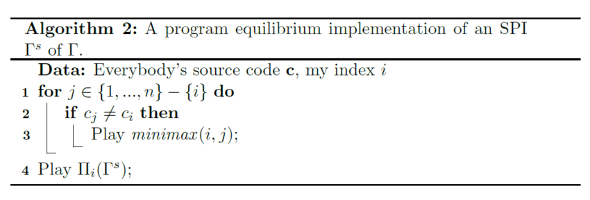
Proposition 18. Let $\Gamma$ be a game and let $\Gamma^s$ be an SPI on $\Gamma$. Let $\mathbf{c}$ be the program profile consisting only of Algorithm 2 for each player. Assume that $\Pi(\Gamma)$ guarantees each player at least threat point utility in expectation. Then $\mathbf{c}$ is a program equilibrium and $\mathit{apply}(\mathbf{c})=\Pi(\Gamma^s)$.

Proof. By inspection of Algorithm 2, we see that $\mathit{exec}(\mathbf{c})=\Pi(\Gamma^s)$. It is left to show that $\mathbf{c}$ is a Nash equilibrium. So let $i$ be any player and $c_i'\in \mathrm{PROG}_i - \{c_i\}$. We need to show that $\mathbb{E}\left[ u_i(\mathit{exec}(\mathbf{c}_{-i},c_i')) \right] \leq \mathbb{E}\left[ u_i(\mathit{exec}(\mathbf{c})) \right]$. Again, by inspection of $\mathbf{c}$, $\mathit{exec}(\mathbf{c}_{-i},c_i')$ is the threat point of Player $i$. Hence,

$$\begin{aligned} \mathbb{E}\left[ u_i(\mathit{exec}(\mathbf{c}_{-i},c_i')) \right] &= v_i\\ &\leq \mathbb{E}\left[ u_i(\Pi(\Gamma)) \right]\\ &\leq \mathbb{E}\left[ u_i(\Pi(\Gamma^s)) \right]\\ &= \mathbb{E}\left[ u_i(\mathit{exec}(\mathbf{c})) \right] \end{aligned}$$

as required.

Theorem 1 follows immediately.

B A discussion of work by Sen (1974) and Raub (1990) on preference adaptation games

We here discuss Raub’s [45] paper in some detail, which in turn elaborates on an idea by Sen [51]. Superficially, Raub’s setting seems somewhat similar to ours, but we here argue that it should be thought of as closer to the work on program equilibrium and bilateral precommitment. In Sections 1, 3 and 3.2, we briefly discuss multilateral commitment games, which have been discussed before in various forms in the gametheoretic literature. Our paper extends this setting by allowing instructions that let the representatives play a game without specifying an algorithm for solving that game. On first sight, it appears that Raub pursues a very similar idea. Translated to our setting, Raub allows that as an instruction, each player $i$ chooses a new utility function $u^s_i\colon A \rightarrow \mathbb{R}$, where $A$ is the set of outcomes of the original game $\Gamma$. Given instructions $u^s_1,...,u^s_n$, the representatives then play the game $(A,\mathbf{u}^s)$. In particular, each representative can see what utility functions all the other representatives have been instructed to maximize. However, what utility function representative $i$ maximizes is not conditional on any of the instructions by other players. In other words, the instructions in Raub's paper are raw utility functions without any surrounding control structures, etc. Raub then asks for equilibria $\mathbf{u}^s$ of the meta-game that Pareto-improve on the default outcome.

To better understand how Raub's approach relates to ours, we here give an example of the kind of instructions Raub has in mind. (Raub uses the same example in his paper.) As the underlying game $\Gamma$, we take the Prisoner's Dilemma. Now the main idea of his paper is that the original players can instruct their representatives to adopt so-called Assurance Game preferences. In the Prisoner's Dilemma, this means that the representatives prefer to cooperate if the other representative cooperates, and prefer to defect if the other player defects. Further, they prefer mutual cooperation over mutual defection. An example of such Assurance Game preferences is given in Table 8. (Note that this payoff matrix resembles the classic Stag Hunt studied in game theory.)

 

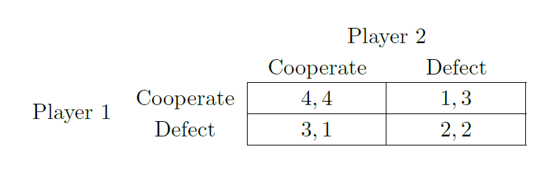
The Assurance Game preferences have two important properties.

1.  If both players tell their representatives to adopt Assurance Game preferences, (Cooperate, Cooperate) is a Nash equilibrium. (Defect, Defect) is a Nash equilibrium as well. However, since (Cooperate, Cooperate) is Pareto-better than (Defect, Defect), the original players could reasonably expect that the representatives play (Cooperate, Cooperate).
2. Under reasonable assumptions about the rationality of the representatives, it is a Nash equilibrium of the meta-game for both players to adopt Assurance Game preferences. If Player 1 tells her representative to adopt Assurance Game preferences, then Player 2 maximizes his utility by telling his representative to also maximize Assurance Game preferences. After all, representative 1 prefers defecting if representative 2 defects. Hence, if Player 2 instructs his representative to adopt preferences that suggest defecting, then he should expect representative to defect as well.

The first important difference between Raub's approach and ours is related to item 2. We have ignored the issue of making SPIs $\Gamma^s$ Nash equilibria of our meta game. As we have explained in Section 3.2 and Appendix A, we imagine that this is taken care of by additional bilateral commitment mechanisms that are not the focus of this paper. For Raub's paper, on the other hand, ensuring mutual cooperation to be stable in the new game $\Gamma^s$ is arguably the key idea. Still, we could pursue the approach of the present paper even when we limit assumptions to those that consist only of a utility function.

The second difference is even more important. Raub assumes that – as in the PD – the default outcome of the game ($\Pi(\Gamma)$ in the formalism of this paper) is known. (Less significantly, he also assumes that it is known how the representatives play under assurance game preferences.) Of course, the key feature of the setting of this paper is that the underlying game $\Gamma$ might be difficult (through equilibrium selection problems) and thus that the original players might be unable to predict $\Pi(\Gamma)$.

These are the reasons why we cite Raub in our section on bilateral commitment mechanisms. Arguably, Raub's paper could be seen as very early work on program equilibrium, except that he uses utility functions as a programming language for representative. In this sense, Raub's Assurance Game preferences are analogous to the program equilibrium schemes of Tennenholtz [55], Oesterheld [55], Barasz et al. [5] and van der Hoek, Witteveen, and Wooldridge [57], ordered in increasing order of similarity of the main idea of the scheme.

C Proof of Lemma 4

Lemma 4. Let $\Phi$ and $\Psi$ be isomorphisms between $\Gamma$ and $\Gamma'$. If $\Phi$ is (strictly) Pareto-improving, then so is $\Psi$.

Proof. 

First, we argue that if $\Phi$ and $\Psi$ are isomorphisms, then they are isomorphisms relative to the same constants $\boldsymbol\lambda$ and $\mathbf c$. For each player $i$, we distinguish two cases. First the case where all outcomes $\mathbf{a}$ in $\Gamma$ have the same utility for Player $i$ is trivial. Now imagine that the outcomes of $\Gamma$ do not all have the same utility. Then let $y_{\mathrm{min}}$ and $y_{\mathrm{max}}$ be the lowest and highest utilities, respectively, in $\Gamma$. Further, let $x_{\mathrm{min}}$ and $x_{\mathrm{max}}$ be the lowest and highest utilities, respectively, in $\Gamma'$. It is easy to see that if $\Psi$ is a game isomorphism, it maps outcomes with utility $y_{\mathrm{min}}$ in $\Gamma$ onto outcomes with utility $x_{\mathrm{min}}$ in $\Gamma'$, and outcomes with utility $y_{\mathrm{max}}$ in $\Gamma$ onto outcomes with utility $x_{\mathrm{max}}$ in $\Gamma'$. Thus, if $\lambda_{\Psi,i}$ and $c_{\Psi,i}$ are to be the constants for $\Psi$, then

$$\begin{aligned} y_{\mathrm{min}} &= \lambda_{\Psi,i}x_{\mathrm{min}} + c_{\Psi,i}\\ y_{\mathrm{max}} &= \lambda_{\Psi,i}x_{\mathrm{max}} + c_{\Psi,i}. \end{aligned}$$

Since $x_{\mathrm{min}}\neq x_{\mathrm{max}}$, this system of linear equations has a unique solution. By the same pair of equations, the constants for $\Phi$ are uniquely determined.

It follows that for all $\mathbf{a}\in A$,

$$\begin{aligned} \mathbf{u}(\mathbf{a}) &= \boldsymbol{\lambda}\mathbf{u}' (\Psi (\mathbf{a}))+\mathbf{c}\\ &= \mathbf{u}(\Phi^{-1}(\Psi(\mathbf{a})))\\ &\leq \mathbf{u}(\Phi (\Phi^{-1}(\Psi(\mathbf{a}))))\\ &= \mathbf{u}(\Psi(\mathbf{a})). \end{aligned}$$

Furthermore, if $\Phi$ is strictly Pareto-improving for some $\tilde {\mathbf{a}} \in A$, then by bijectivity of $\Phi,\Psi$, there is $\mathbf{a}\in A$ s.t. $\Phi^{-1}(\Psi(\mathbf{a}))=\tilde {\mathbf{a}}$. For this $\mathbf{a}$, the inequality above is strict and therefore $\mathbf{u}(\mathbf{a})< \mathbf{u}(\Psi(\mathbf{a}))$.

D Proof of Theorem 9

We here prove Theorem 9. We assume familiarity with basic ideas in computational complexity theory (non-deterministic polynomial time (NP), reductions, NP-completeness, etc.).

D.1 On the structure of relevant outcome correspondence sequences

Throughout our proof we will use a result about the structure of relevant outcome correspondences. Before proving this result, we give two lemmas. The first is a well-known lemma about elimination by strict dominance.

Lemma 19 (path independence of iterated strict dominance). Let $\Gamma$ be a game in which some strategy $a_i$ of player $i$ is strictly dominated. Let $\Gamma'$ be a game we obtain from $\Gamma$ by removing a strictly dominated strategy (of any player) other than $a_i$. Then $a_i$ is strictly dominated in $\Gamma'$.

Note that this lemma does not by itself prove that iterated strict dominance is path dependence. However, path independence follows from the property shown by this lemma.

Proof. Let $a_i'$ be the strategy that strictly dominates $a_i$. We distinguish two cases:

Case 1: The strategy removed is $a_i'$. Then there must be $\hat a_i$ that strictly dominates $a_i'$. Then it is for all $a_{-i}$

$$\begin{equation*} u_i(\hat a_i,a_{-i})> u_i( a_i',a_{-i})>u_i(a_i,a_{-i}). \end{equation*}$$

Both inequalities are due to the definition of strict dominance. We conclude that $\hat a_i$ must strictly dominate $a_i$.

Case 2: The strategy removed is one other than $a_i$ or $a_i'$. Since the set of strategies of the new game is a subset of the strategies of the old game it is still for each strategy $a_{-i}$ in the new game

$$\begin{equation*} u_i(a_i',a_{-i})>u_i(a_i,a_{-i}), \end{equation*}$$

i.e., $a_i'$ still strictly dominates $a_i$.

The next lemma shows that instead of first applying Assumption 1 plus symmetry (Lemma 2.2) to add a strictly dominated action and then applying Assumption 1 to eliminate a different strictly dominated strategy, we could also first eliminate the strictly dominated strategy and then add the other strictly dominated strategy.

Lemma 20. Let $\Gamma \sim_{\left( \Phi^{\mathrm{red}} \right)^{-1}} \hat\Gamma$ by Assumption 1, where $\Gamma$ is the reduced game, and $\hat\Gamma\sim_{\tilde\Phi^{\mathrm{red}}}\tilde\Gamma$ by Assumption 1. Then either $\Gamma=\hat\Gamma$ or there is a game $\Gamma'$ s.t. $\Gamma\sim_{\tilde\Phi^{\mathrm{red}}} \Gamma'$ by Assumption 1 and $\Gamma'\sim_{\left( \Phi^{\mathrm{red}} \right)^{-1}} \tilde\Gamma$ by Assumption 1.

Proof. By the assumption both $\tilde\Gamma$ and $\Gamma$ can be obtained from eliminating a strictly dominated action from $\hat\Gamma$. Let these actions be $\tilde a$ and $a$, respectively. If $\tilde a = a$, then $\Gamma=\tilde\Gamma$. So for the rest of this proof assume $\tilde a\neq a$. Let $\Gamma'$ be the game we obtain by removing $\tilde a$ from $\Gamma$. We now show the two outcome correspondences:

• First we show that $\Gamma\sim_{\tilde\Phi^{\mathrm{red}}} \Gamma'$, i.e., that $\tilde a$ is strictly dominated in $\Gamma$. For this notice that $\tilde a$ and $a$ are both strictly dominated in $\hat\Gamma$. Now $\Gamma$ is obtained from $\hat\Gamma$ by removing $a$. By Lemma 19, $\tilde a$ is still strictly dominated in $\Gamma$, as claimed.
• Second we show that $\Gamma'\sim_{\left( \Phi^{\mathrm{red}} \right)^{-1}} \tilde\Gamma$, i.e., that $\tilde\Gamma \sim_{\Phi^{\mathrm{red}}} \Gamma'$, i.e., that $a$ is strictly dominated in $\tilde\Gamma$. Recall again that $\tilde a$ and $a$ are both strictly dominated in $\hat\Gamma$. Now $\tilde\Gamma$ is obtained from $\hat\Gamma$ by removing $a$. By Lemma 19, $a$ is still strictly dominated in $\tilde\Gamma$, as claimed.

We are ready to state our lemma about the structure of outcome correspondences.

Lemma 21. Let

$$\begin{equation*}\Gamma^1\sim_{\Phi ^1} ... \sim_{\Phi ^{k-1}} \Gamma^k,\end{equation*}$$

where each outcome correspondence is due to a single application of Assumption1, Assumption1 plus symmetry (Lemma 2.2) or Assumption 2. Then there is a sequence $\Gamma'^1,...,\Gamma'^m$ with $\Gamma'^1=\Gamma^1$ and $\Gamma'^m=\Gamma^m$, $m\leq k$ and $l$ such that

$$\begin{equation*}\Gamma^1\sim_{\Psi^1} \Gamma ^{\prime 2} \sim_{\Psi^2} \Gamma ^{\prime 3} \sim_{\Psi^3} ... \sim_{\Psi^{l-1}} \Gamma ^ {\prime l}\end{equation*}$$

all by single applications of Assumption 1, $\Gamma ^ {\prime l}$ and $\Gamma ^{\prime l+1}$ are fully reduced games such that $\Gamma ^ {\prime l} \sim_{\Psi^{l}} \Gamma ^{\prime l+1}$ by a single application of Assumption 2, and

$$\begin{equation*}\Gamma^{\prime l+1}\sim_{\left(\Psi^{l+1}\right)^{-1}} \Gamma ^{\prime l+ 2} \sim_{\left(\Psi^{\prime l+2}\right)^{-1}} ... \sim_{\left(\Psi^{\prime m}\right)^{-1}} \Gamma ^ {\prime m}\end{equation*}$$

all by single applications of Assumption 1 with Lemma 2.2.

A conciser way to state the consequence is that there must be games $\Gamma^{\mathrm{red}}$, $\Gamma^{s,\mathrm{red}}$ and $\Gamma^s$ such that $\Gamma^{\mathrm{red}}$ is obtained from $\Gamma$ by iterated elimination of strictly dominated strategies, $\Gamma^{s,\mathrm{red}}$ is isomorphic to $\Gamma^{s,\mathrm{red}}$, and $\Gamma^{s,\mathrm{red}}$ is obtained from $\Gamma^s$ by iterated elimination of strictly dominated strategies.

Proof.  First divide the given sequence of outcome correspondences up into periods that are maximally long while containing only correspondences by Assumption 1 (with or without Lemma 2.2). That is, consider subsequences of the form $\Gamma^q\sim_{\Phi^q} ... \sim_{\Phi^{r-1}}\Gamma^r$ such that:

• Each of the correspondences $\Gamma^q\sim_{\Phi^q} \Gamma^{q+1}$, ..., $\Gamma^{r-1}\sim_{\Phi^{r-1}}\Gamma^r$ is by applying Assumption 1 with or without Lemma 2.2.
• Either $q=1$ or the correspondence $\Gamma^{q-1}\sim_{\Phi^{q-1}}\Gamma^q$ is by Assumption 2.
• Either $r=k$ or the correspondence $\Gamma^{r}\sim_{\Phi^{r}}\Gamma^{r+1}$ is by Assumption 2.

In each such period apply Lemma 20 iteratively to either eliminate or move to the right all inverted reduction elimination steps.

In all but the first period, $\Gamma^q$ contains no strictly dominated actions (by stipulation of Assumption 2). Hence all but the first period cannot contain any non-reversed elimination steps. Similarly, in all but the final period, $\Gamma^r$ contains no strictly dominated actions. Hence, in all but the final period, there can be no reversed applications of Assumption 1.

Overall, our new sequence of outcome correspondences thus has the following structure: first there is a sequence of elimination steps via Assumption 1, then there is a sequence of isomorphism steps, and finally there is a sequence of reverse elimination steps. We can summarize all the applications of Assumption 2 into a single step applying that assumption to obtain the claimed structure.

Now notice that that the reverse elimination steps are only relevant for deriving unilateral SPIs. Using the above concise formulation of the lemma, we can always simply use $\Gamma^{s,\mathrm{red}}$ itself as an omnilateral SPI – it is not relevant that there is some subset game $\Gamma^s$ that reduces to $\Gamma^{s,\mathrm{red}}$.

Lemma 22. As in Lemma 21, let $\Gamma^1\sim_{\Phi ^1} ... \sim_{\Phi ^{k-1}} \Gamma^k$, where each outcome correspondence is due to a single application of Assumption 1, Assumption 1 plus symmetry (Lemma 2.2) or Assumption 2. Let $\Gamma^2,...,\Gamma^k$ all be subset games of $\Gamma^1$. Moreover, let $\Phi^{k-1}\circ ... \circ \Phi^1$ be Pareto improving. Then there is a sequence of subset games $\Gamma'^2,...,\Gamma'^m,\Gamma'^{m+1}$ such that $\Gamma^1\sim_{\Psi^1}\Gamma'^2\sim_{\Psi^2}...\sim_{\Psi^{m-1}}\Gamma'^m$ all by applications of Assumption 1 (without applying symmetry), and $\Gamma'^m\sim_{\Xi} \Gamma'^{m+1}$ by application of Assumption 2 such that $\Xi\circ \Psi^{m-1}...\circ \Psi^1$ is Pareto improving.

Proof. First apply Lemma 21. Then notice that the correspondence functions from applying Assumption 1 with symmetry have no effect on whether the overall outcome correspondence is Pareto improving.

D.2 Non-deterministic polynomial-time algorithms for the SPI problem

D.2.1 The omnilateral SPI problem

We now show that the SPI problem is in NP at all. The following algorithm can be used to determine whether there is a safe Pareto improvement: Reduce the given game $\Gamma$ until it can be reduced no further to obtain some subset game $\Gamma'=(A',\mathbf{u})$. Then non-deterministically select injections $\Phi_i\colon A_i' \rightarrow A_i$. If $\Phi=(\Phi_1,...,\Phi_n)$ is (strictly) Pareto-improving (as required in Theorem 3), return True with the solution $\Gamma^s$ defined as follows: The set of action profiles is defined as $A^s=\bigtimes_i \Phi_i(A_i')$. The utility functions are

$$\begin{equation*} u_i^s\colon A^s \rightarrow \mathbb{R} \colon \mathbf{a}^s \mapsto (u_i(\Phi_1^{-1}(a_1^s),...,\Phi_n^{-1}(a_n^s)))_{i=1,...,n}. \end{equation*}$$

Otherwise, return False.

Proposition 23. The above algorithm runs in non-deterministic polynomial time and returns True if and only if there is a (strict) unilateral SPI.

Proof. It is easy to see that this algorithm runs in non-deterministic polynomial time. Furthermore, with Lemma: 4 it is easy to see that if this algorithm finds a solution $\Gamma^s$, that solution is indeed a safe Pareto improvement. It is left to show that if there is a safe Pareto improvement via a sequence of Assumption 1 and 2 outcome correspondences, then the algorithm indeed finds a safe Pareto improvement.

Let us say there is a sequence of outcome correspondences as per AssumptionS 1 and 2 that show $\Gamma\sim_{\Phi} \Gamma^s$ for Pareto-improving $\Phi$. Then by Lemma 22, there is $\Gamma'$ such that $\Gamma\sim_{\Psi^{\mathrm{red}}} \Gamma'$ via applying Assumption 1 iteratively to obtain a fully reduced $\Gamma'$ and $\Gamma'\sim_{\Psi^{\mathrm{iso}}} \Gamma ^s$ via a single application of Assumption 2. By construction, our algorithm finds (guesses) this Pareto-improving outcome correspondence.

Overall, we have now shown that our non-deterministic polynomial-time algorithm is correct and therefore that the SPI problem is in NP. Note that the correctness of other algorithms can be proven using very similar ideas. For example, instead of first reducing and then finding an isomorphism, one could first find an isomorphism, then reduce and then (only after reducing) test whether the overall outcome correspondence function is Pareto-improving. One advantage of reducing first is that there are fewer isomorphisms to test if the game is smaller. In particular, the number of possible isomorphisms is exponential in the number of strategies in the reduced game $\Gamma '$ but polynomial in everything else. Hence, by implementing our algorithm deterministically, we obtain the following positive result.

Proposition 24. For games $\Gamma$ with $|A_1|+...+|A_n|=m$ that can be reduced (via iterative application of Assumption 1) to a game $\Gamma'$ with $|A_1'|+...+|A_n'|=l$, the (strict) omnilateral SPI decision problem can be solved in $O(m^l)$.

D.2.2 The unilateral SPI problem

Next we show that the problem of finding unilateral SPIs is also in NP. Here we need a slightly more complicated algorithm: We are given an $n$-player game $\Gamma$ and a player $i$. First reduce the game $\Gamma$ fully to obtain some subset game $\Gamma^{\mathrm{red}}$. Then non-deterministically select injections $\Phi_i\colon A_i^{\mathrm{red}} \rightarrow A_i$. The resulting candidate SPI game then is

$$\begin{equation*} \Gamma^s=((A_{-i},\Phi_i(A_i^{\mathrm{red}})),(\mathbf{u}_{-i},u_i^s)), \end{equation*}$$

where $u_i^s(\mathbf{a}^s)=u_i(\Phi^{-1}_1(a^s_1),...,\Phi^{-1}_n(a^s_n))$ for all $\mathbf{a}^s\in \Phi(A^{\mathrm{red}})$, and $u_i^s(\mathbf{a}^s)$ is arbitrary for $\mathbf{a}^s\notin \Phi(A^{\mathrm{red}})$. Return True if the following conditions are satisfied:

1. The correspondence function $\Phi$ must be (strictly) Pareto improving (as per the utility functions $\mathbf{u}$).
2. For each $j\in\{1,...,n\}-\{ i \}$, there are $\lambda_j\in\mathbb{R}_+$ and $c_j\in\mathbb{R}$ such that for all $\mathbf{a}\in A^{\mathrm{red}}$, we have $u_j(\mathbf{a})=\lambda_j u_j(\Phi(\mathbf{a}))+c_j$.
3. The game $\Gamma^s$ reduces to the game $(\Phi(A^{\mathrm{red}}),(\mathbf{u}_{-i},u_i^s))$.

Otherwise, return False.

Proposition 25. The above algorithm runs in non-deterministic polynomial time and returns True if and only if there is a (strict) unilateral SPI.

Proof. First we argue that the algorithm can indeed be implemented in non-deterministic polynomial time. For this notice that for checking Item 2, the constants can be found by solving $n$ systems of linear equations of two variables.

It is left to prove correctness, i.e., that the algorithm returns True if and only if there exists an SPI. We start by showing that if the algorithm returns True, then there is an SPI. Specifically, we show that if the algorithm returns True, the game $\Gamma^s$ is indeed an SPI game. Notice that $\Gamma\sim_{\Psi}\Gamma^{\mathrm{red}}$ for some $\Psi$ by iterative application of Assumption 1 with Transitivity (Lemma 2.2); that $\Gamma^{\mathrm{red}} \sim_{\Phi} (\Phi(A^{\mathrm{red}}),(\mathbf{u}_{-i},u_i^s))$ by application of Assumption 2. Finally, $(\Phi(A^{\mathrm{red}}),(\mathbf{u}_{-i},u_i^s))\sim_{\Xi^{-1}} \Gamma^s$ for some $\Xi$ by iterative application of Assumption 1 to $\Gamma^s$, plus transitivity (Lemma 2.3) with reversal (Lemma 2.2).

It is left to show that if there is an SPI, then the above algorithm will find it and return true. To see this, notice that Lemma 21 implies that there is a sequence of outcome correspondences $\Gamma\sim_{\Psi}\Gamma^{\mathrm{red}}\sim_{\Phi}\Gamma^{s,\mathrm{red}}\sim_{\Xi} \Gamma^s$. We can assume that $\Gamma^{s,\mathrm{red}}$ and $\Gamma^s$ have the same action sets for Player $i$. It is easy to see that in $\Gamma^s$ we could modify the utilities $u^s_i(\mathbf{a})$ for any $\mathbf{a}$ that is not in $\Gamma^{s,\mathrm{red}}$, because Player $i$'s utilities do not affect the elimination of strictly dominated strategies from $\Gamma^s$.

Proposition 26. For games $\Gamma$ with $|A_1|+...+|A_n|=m$ that can be reduced (via iterative application of Assumption 1) to a game $\Gamma'$ with $|A_1'|+...+|A_n'|=l$, the (strict) unilateral SPI decision problem can be solved in $O(m^l)$.

D.3 The SPI problems are NP-hard

We now proceed to showing that the safe Pareto improvement problem is NP-hard. We will do this by reducing the subgraph isomorphism problem to the (two-player) safe Pareto improvement problem. We start by briefly describing one version of that problem here.

A (simple, directed) graph is a tuple $(n,a\colon \{1,...,n\} \times \{1,...,n\} \rightarrow \mathbb{B})$, where $n\in \mathbb{N}$ and $\mathbb{B}\coloneqq\{0,1\}$. We call $a$ the adjacency function of the graph. Since the graph is supposed to be simple and therefore free of self-loops (edges from one vertex to itself), we take the values $a(j,j)$ for $j\in \{1,...,n\}$ to be meaningless.

For given graphs $G=(n,a)$,$G'=(n',a')$ a subgraph isomorphism from $G$ to $G'$ is an injection $\phi\colon \{1,...,n\} \rightarrow \{ 1,...n'\}$ such that for all $j\neq l$

$$\begin{equation*} a(j,l)\leq a'(\phi(j),\phi(l)). \end{equation*}$$

In words, a subgraph isomorphism from $G$ to $G'$ identifies for each node in $G$ a node in $G'$ s.t. if there is an edge from node $j$ to node $l$ in $G$, there must also be an edge in the same direction between the corresponding nodes $\phi(j),\phi(l)$ in $G'$. Another way to say this is that we can remove some set of ($n'-n$) nodes and some edges from $G'$ to get a graph that is just a relabeled (isomorphic) version of $G$.

Definition 8. Given two graphs $G,G'$, the subgraph isomorphism problem consists in deciding whether there is a subgraph isomorphism $\phi$ between $G,G'$.

The following result is well-known.

Lemma 27 ([12, Theorem 2]). The subgraph isomorphism problem is NP-complete.

Lemma 28. The subgraph isomorphism problem is reducible in linear time with linear increase in problem instance size to the (strict) (unilateral) safe Pareto improvement problem for two players. As a consequence, the (strict) (unilateral) safe Pareto improvement problem is NP-hard.

Proof. Let $G=(n,a)$ and $\hat G=(\hat n,\hat a)$ be graphs. Without loss of generality assume both graphs have at least $2$ vertices, i.e., that $n,\hat n\geq 2$. For this proof, we define $[i]\coloneqq \{1,...,i\}$ for any $i\in \mathbb{N}$.

We first define two games, one for each graph, and then a third game that contains the two.

The game for $G$ is the game $\Gamma$ as in Table 9. Formally, let $\epsilon<\nicefrac{1}{2n}$. Then we let $\Gamma=(A_1,A_2,u_1,u_2)$, where $A_1=A_2=[2n+2]$. The utility functions are defined via

$$\begin{equation*} u_1(i,j) = \left\{\begin{array}{cl} 2, & \text{if } i=j\text{ and }i,j\in[n]\\ a(i,j), & \text{if }i\neq j \text{ and }i,j\in[n]\\ -1, & \text{if } i\in \{ n+1,...,2n\},j\in[n]\text{ and }i\neq j+n \\ -1, & \text{if } i\in [n],j\in\{n+1,...,2n\}\text{ and }i+n\neq j \\ 4+(n+i)\epsilon & \text{if } i\in [n]\text{ and }j=i+n \\ 4+j\epsilon & \text{if } j\in[n]\text{ and }i= j+n \\ -1 & \text{if } i,j\in \{ n+1,...,2n\}\\ 3 & \text{if }i\in \{ 2n+1,2n+2\}\text{ and }j\in [2n]\\ 6 & \text{if }i=j=2n+1\\ \epsilon & \text{if }j\in\{2n+1,2n+2\} \text{ and not }i=j=2n+1 \end{array}\right. \end{equation*}$$

and

$$\begin{equation*} u_2(i,j) = \left\{\begin{array}{cl} 2, & \text{if } i=j\text{ and }i,j\in[n]\\ 1, & \text{if }i\neq j \text{ and }i,j\in[n]\\ -1, & \text{if } i\in \{ n+1,...,2n\},j\in[n]\text{ and }i\neq j+n \\ -1, & \text{if } i\in [n],j\in\{n+1,...,2n\}\text{ and }i+n\neq j \\ 4 & \text{if } i\in [n]\text{ and }j=i+n \\ 4 & \text{if } j\in[n]\text{ and }i= j+n \\ -1 & \text{if } i,j\in \{ n+1,...,2n\}\\ 3 & \text{if }j\in \{ 2n+1,2n+2\}\text{ and }i\in [2n]\\ 6 & \text{if }i=j=2n+2\\ \epsilon & \text{if }i\in\{2n+1,2n+2\} \text{ and not }i=j=2n+2 \end{array}\right.. \end{equation*}$$

We define $\hat\Gamma$ based on $\hat G$ analogously, except that in Player 1's utilities we use $5$ instead of $4$, $5+(n+i)\epsilon$ instead of $4+(n+i)\epsilon$, $5+j\epsilon$ instead of $4+j\epsilon$ and $4$ instead of $3$.

 

 

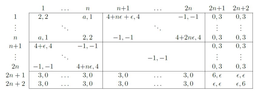
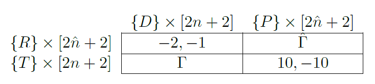
We now define $\Gamma^c=(A^c,\mathbf{u}^c)$ from $\Gamma$ and $\hat\Gamma$ as sketched in Table 9. For the following let

$$\begin{aligned} A^{\Gamma} &= (\{ T \} \times [2n+2])\times (\{ D \} \times [2n+2] )\\ A^{\hat\Gamma}&= (\{ R \} \times [2\hat n +2])\times (\{ P \} \times [2\hat n + 2]), \end{aligned}$$

and $A_1^c=A_1^{\Gamma} \cup A_1^{\hat\Gamma}$ and $A_2^c=A_2^{\Gamma} \cup A_2^{\hat\Gamma}$. For $i,j\in [2n+2]$, let $\mathbf{u}^c((T,i),(D,j))$ be the utility of $(i,j)$ in $\Gamma$. For $i,j\in [2\hat n+2]$ let $\mathbf{u}^c((R,i),(P,j))$ be the utility of $(i,j)$ in $\hat\Gamma$. Finally, define $\mathbf{u}^c((R,i),(D,j))=(-2,-1)$ for all $i\in [2\hat n+2]$ and all $j\in [2n+2]$; and $\mathbf{u}^c((T,i),(P,j))=(10,-10)$ for all $i\in [2 n+2]$ and all $j\in [2\hat n+2]$.

It is easy to show that this reduction can be computed in linear time and that it also increases the problem instance size only linearly.

To prove our claim, we need to prove the following two propositions:

1. If there is a subgraph isomorphism from $G$ to $\hat G$, then there is a unilateral, strict SPI.
2. If there is any SPI, then there is a subgraph isomorphism from $G$ to $\hat G$.

1. We start with the first claim. Assume there is a subgraph isomorphism $\phi$ from $G$ to $G'$. We construct our SPI as usual: first we reduce the game $\Gamma^c$ by iterated elimination of strictly dominated strategies, then we find a Pareto-improving outcome equivalence between the reduced game and some subset game $\Gamma^{s,\mathrm{red}}$ of $\Gamma^c$. Finally, we show that $\Gamma^{s,\mathrm{red}}$ arises from removing strictly dominated strategies from subset game $\Gamma^s$ of $\Gamma^c$. It is easy to see that the game resulting from iterated elimination of strictly dominated strategies is just the $\Gamma$ part of it. Abusing notation a little, we will in the following just call this $\Gamma$ (even though it has somewhat differently named action sets).

Next we define a pair of functions $\Psi_{1/2}$, which will later form our isomorphism. For all $i\in [n]$ and $b\in \{1,2\}$, we define $\Psi_1$ via

$$\begin{aligned} \Psi_{1}(T,i) &= (R,\phi(i))\\ \Psi_1(T,n+i) &= (R,\hat n + \phi(i))\\ \Psi_1(T,2n+b) &= (R,2\hat n + b) \end{aligned}$$

Define $\Psi_2(D,i) = (P,\phi(i))$ and so on analogously.

Now define $\Gamma^{s,\mathrm{red}}$ to be the subset game with action sets $\Psi_{1}(A_1)$ and $\Psi_2(A_2)$, where $A_1$ and $A_2$ are the action sets of $\Gamma$; and with utility functions

$$\begin{equation*} u_1^s\colon \Psi_{1}(A_1) \times \Psi_2(A_2)\rightarrow \mathbb{R}\colon \mathbf{a}^s \mapsto u_1^c(\Psi^{-1}(\mathbf{a}^s)) \end{equation*}$$

and $u_2^c$ (as restricted to $\Psi_{1}(A_1) \times \Psi_2(A_2)$).

We must now show that $\Psi$ is a game isomorphism between $\Gamma$ and $\Gamma^{s,\mathrm{red}}$. First, it is easy to see that for $i=1,2$, $\Psi_i$ is a bijection between $A_i$ and $\Psi_i(A_i)$. Moreover,

$$\begin{equation*} u_1^s(\Psi(\mathbf{a})) = u_1^c(\Psi^{-1}(\Psi(\mathbf{a}))) = u^c_1(\mathbf{a}). \end{equation*}$$

For player 2, we need to distinguish the different cases of actions. Since each case is trivial from looking at the definition of $\Gamma$ and $\hat\Gamma$ we omit the detailed proof.

Next we need to show that $\Psi$ is strictly Pareto-improving as judged by the original players' utility function $u^c$. Again, this is done by distinguishing a large number of cases of action profiles $\mathbf{a}$, all of which are trivial on their own. The most interesting one is that of $((T,i),(D,j))$ for $i,j\in [n]$ with $i\neq j$ because this is where we use the fact that $\phi$ is a subgraph isomorphism:

$$\begin{aligned} u^c_1(\Psi((T,i),(D,j))) &= u^c_1((R,\phi(i)),(P,\phi(j)))\\ &= \hat a(\phi(i),\phi(j))\\ &\geq a (i,j)\\ &= u_1^c((T,i),(D,j)). \end{aligned}$$

We omit the other cases.

It is left to construct a unilateral subset game $\Gamma^{s}$ of $\Gamma^c$ such that $\Gamma^s$ reduces to $\Gamma^{s,\mathrm{red}}$ via iterated elimination of strictly dominated strategies. Let $\Gamma^s=(\Psi_1(A_1),A_2^c,u_1^s,u_2^c)$, where we set $u_1^s(a_1,a_2)$ arbitrarily for $a_2\in A_2^c-\Psi_2(A_2)$.

We now show that $\Gamma^s$ reduces to $\Gamma^{s,\mathrm{red}}$ via repeated application of Assumption 1. So let $a_2\in A_2^c-\Psi_2(A_2)$. We distinguish the following cases:

• If $a_2\in D\times [2n+2]$, then $a_2$ is strictly dominated by $(P,2\hat n +1)$ and by $(P,2\hat n +2)$.
• If $a_2=(P,i)$ for some $i\in \{1,...,\hat n\}$, then by assumption that $a_2\in A_2^c-\Psi(A_2)$ and by construction of $\Psi$, we know that $(R,n+i)\notin \Psi_1(A_1)$. From this and inspecting Table 9 we see that $(P,2\hat n +1)$ and $(P,2\hat n+2)$ strictly dominate $(P,i)$.
• If $a_2=(P,\hat n + i)$ for some $i\in \{1,...,\hat n\}$, then by assumption that $a_2\in A_2^c-\Psi_2(A_2)$ and by construction of $\Psi$, we know that $(R,i)\notin \Psi_1(A_1)$. From this and inspecting Table 9 we see that $(P,2\hat n +1)$ and $(P,2\hat n+2)$ strictly dominate $(P,\hat n +i)$.

Note that $(P,2\hat n +1)$ and $(P,2\hat n + 2)$ are both in $\Psi_2(A_2)$ by construction of $\Psi$.

2. It is left to show that if there is any kind of non-trivial SPI, there is also a subgraph isomorphism from $G$ to $\hat G$.

By Lemma 21, if there is an SPI, there are bijections $\Psi_1,\Psi_2$ that are jointly Pareto-improving from the reduced game $\Gamma$ to $\Gamma^c$. From these functions we will construct a subgame isomorphism. However, to do so (and to see that the resulting function is indeed a subgraph isomorphism), we need to first make a few simple observations about the structure of $\Psi_1$ and $\Psi_2$. Define $A^{\Gamma,[n]}=(\{ T \} \times [n])\times (\{ D \} \times [n])$ and $A^{\hat\Gamma,[\hat n]}=(\{ R \} \times [\hat n])\times (\{ P \} \times [\hat n])$.

1.  First we will argue that there is an action $\mathbf{a}\in A^{\Gamma}$ of the reduced game s.t. $\Psi(\mathbf{a})\in A^{\hat \Gamma}$. We prove this by showing the following contrapositive: if $\Psi(A^\Gamma)$ and $A^{\hat \Gamma}$ are disjoint, then $\Psi$ must, contrary to assumption, be trivial, i.e., $\Psi$ must be the pair of identity functions on $A^\Gamma$.From the fact that $\Psi$ is Pareto improving, it follows that $\Psi((T,2n+1),(D,2n+1))=((T,2n+1),(D,2n+1))$, since outside of $A^{\hat \Gamma}$ there is no outcome with utility at least $6$ for Player $1$. Similarly,

   $$\Psi((T,2n+2),(D,2n+2))=((T,2n+2),(D,2n+2)).$$

   It then follows that $\Psi((T,n),(D,2n))=((T,n),(D,2n))$, since apart from the outcomes we have already mapped to, no other outcome gives Player $1$ a utility of $4+2n\epsilon$. Next it follows that $\Psi((T,n-1),(D,2n-1))=((T,n-1),(D,2n-1))$, again because all outcomes with utility at least $4+(2n-1)\epsilon$ for Player $1$ outside of $A^{\hat \Gamma}$ are already mapped to. And so on, until we obtain that $\Psi((T,1),(D,n+1))=((T,1),(D,n+1))$. By an analogous line of argument we can show that

   $$\Psi((T,2n),(D,n))=((T,2n),(D,n)), ..., \Psi((T,n+1),(D,1))=((T,n+1),(D,1)).$$

   Together these equalities uniquely specify $\Psi_1=\mathrm{id}$ and $\Psi_2=\mathrm{id}$.

2. We next argue that $\Psi (A^{\Gamma}) \subseteq A^{\hat \Gamma}$. We show a contrapositive, specifically that if this were not the case then $\Psi$ would not be Pareto-improving. So assume that $\Psi (A^{\Gamma}) \not\subseteq A^{\hat \Gamma}$. Then from item a it follows that there is $\mathbf{a}\in A^\Gamma$ such that neither $\Psi(\mathbf a)\in A^{\hat \Gamma}$ nor $\Psi(\mathbf a)\in A^{\Gamma}$. Then either $u_1^c(\Psi(\mathbf a))=-2$ and hence $u_1^c(\mathbf{a})>u_1^c(\Psi(\mathbf{a}))$ or $u_2(\Psi(\mathbf a))=-10$ and hence $u_2^c(\mathbf a)<u_2^c(\Psi(\mathbf a))$.

3. We now argue that for $\Psi$ to be Pareto-improving, $\Psi(A^{\Gamma,[n]})$ must be a subset of $A^{\hat \Gamma,[\hat n]}$. To show this, notice first that $\Psi((T,2n+i),(D,2n+j))=((R,2\hat n+i),(P,2\hat n +j))$ for all $i,j\in\{1,2\}$ by a similar argument as used repeatedly in Item a. Hence, $\Psi(A^{\Gamma,[n]}) \subseteq A^{\hat \Gamma, [2n]}$. Now assume for contraposition that there is $i\in [n]$ such that WLOG $\Psi_1(T,i)=(R,j)$ for some $j\in \{\hat n +1,...,2\hat n\}$. Then for all but one opponent move $(D,l)$ with $l\in [2n]$, $u_1^c(\Psi((T,i),(D,l)))=-1$. But since $n\geq 2$, there are at least two opponent moves $(D,l)$ with $l\in [2n]$ such that $u_1^c ((T,i),(D,l))\geq 0$. Hence, $\Psi$ cannot be Pareto-improving.

4. Finally, notice that for $i\in [n]$ and $j\in [\hat n]$, if $\Psi_1(T,i)=(R,j)$, then also $\Psi_2(D,i)=(P,j)$. To see this, assume it was $\Psi_2(R,i)=(P,l)$ for some $l\neq j$. Then by Item c, $l\in [n]$. Hence,

   $$u_2^c((T,i),(R,i))=2>1=u_2^c((R,j),(P,l))=u_2^c(\Psi_1(T,i),\Psi_2(R,i))$$

   in contradiction to the assumption that $\Psi$ is Pareto improving.

We are ready to construct our subgraph isomorphism. For $i\in [n]$, define $\phi(i)$ to be the second element of the pair $\Psi_1(T,i)$. By Item c, $\phi(i)$ can equivalently be defined as the second item in the pair $\Psi_2(D,i)$. By Item d, $\phi$ is a function from $[n]$ to $[\hat n]$. By assumption about $\Psi$, $\phi$ is injective. Further, by construction of $\Gamma^c$ and $\phi$, as well as the assumption that $\Psi$ is Pareto improving, we infer that for all $i,j\in[n]$ with $i\neq j$,

$$\begin{aligned} \hat a (\phi(a), \phi (j)) &= u_1^c ((R,\phi(i)),(P,\phi(j)))\\ &= u_1^c (\Psi_1(T,i),\Psi_2(D,j))\\ &\geq u_1^c((T,i),(D,j))\\ &= a(i,j). \end{aligned}$$

We conclude that $\phi$ is a subgraph isomorphism.

E Proof of Theorem 15

Proof. We will give the proof based on the graphs as well, without giving all formal details. Further we assume in the following that neither $L_1$ nor $L_3$ consist of just a single point, since these cases are easy.

\underline{Case A}: Note first that by Corollary 14 it is enough to show that if ${\mathbf{y}}$ is in any of the listed sets $L_1,L_2,L_3$, it can be made safe.

It's easy to see that all payoff vectors on the curve segment of the Pareto frontier $L_2$ are safely achievable. After all, all payoff vectors in this set Pareto-improve on all outcomes in $\mathrm{supp}(\Pi(\Gamma))$. Hence, for each ${\mathbf{y}}$ on the line segment, one could select the $\Gamma^s$ where ${\mathbf{u}}^e={\mathbf{y}}$.

It is left to show that all elements of $L_{1/2}$ are safely achievable. Remember that not all payoff vectors on the line segments are Pareto improvements, only those that are to the north-east of (Pareto-better than) the default utility. In the following, we will use $L_1'$ and $L_3'$ to denote those elements of $L_1$ and $L_3$, respectively, that are Pareto-improvements on the default.

We now argue that the Pareto improvement ${\mathbf{y}}$ on the line $L_1$ for which $y_1=\mathbb{E}\left[u_1(\Pi(\Gamma))\right]$ is safely achievable. In other words, ${\mathbf{y}}$ is the projection northward of the default utility, or ${\mathbf{y}}=\pi_1(\mathbb{E}\left[{\mathbf{u}}(\Pi(\Gamma))\right],L_1)$. This ${\mathbf{y}}$ is also one of the endpoints of $L_1'$. To achieve this utility, we construct the equivalent game as per Lemma 13, where the utility to the original players of each outcome $(\hat a_1,\hat a_2)$ of the new game $\Gamma^s$ is similarly the projection northward onto $L_1$ of the utility of the corresponding outcome $(a_1,a_2)$ in $\Gamma^s$. That is,

$$\begin{equation*} {\mathbf{u}}^e (\hat a_1,\hat a_2) = \pi_1( {\mathbf{u}}(a_1,a_2),L_1). \end{equation*}$$

Note that because $\mathcal{C}(\Gamma)$ is convex and the endpoints of the line segment $L_1$ are by definition in $\mathcal{C}(\Gamma)$, it is $L_1 \subseteq \mathcal{C}(\Gamma)$. Hence, all values of ${\mathbf{u}}^e$ thus defined are feasible. Because all outcomes in the original game lie below the line $L_1$, $\pi_1$ is linear. Hence,

$$\begin{aligned} \mathbb{E}\left[ {\mathbf{u}}^e (\Pi(\Gamma^s)) \right] &= \mathbb{E}\left[ \pi_1({\mathbf{u}}(\Pi(\Gamma)) , L_1) \right]\\ &= \pi_1(\mathbb{E} \left[ {\mathbf{u}}(\Pi(\Gamma)) \right],L_1) \end{aligned}$$

as required.

We have now shown that one of the endpoints of $L_1'$ is safely achievable. Since the other endpoint of $L_1'$ is in $L_2$, it is also safely achievable. By Corollary 14, this implies that all of $L_1'$ is safely achievable.

By an analogous line of reasoning, we can also show that all elements of $L_3'$ are safely achievable.

\underline{Case B}: Define $L_1',L_3'$ as before as those elements of $L_1,L_3$ respectively that Pareto improve on the default $\mathbb{E}\left[{\mathbf{u}}(\Pi(\Gamma))\right]$. By a similar argument as before, one can show that the utilities $\pi_i(\mathbb{E}\left[{\mathbf{u}}(\Pi(\Gamma))\right],L_j')$ is safely achievable both for $i=1,j=1$ and for $i=2,j=3$. Call these points $E_1$ and $E_3$, respectively.

We now proceed in two steps. First, we will show that there is a third safely achievable utility point $E_2$, which is above both $L_1$ and $L_3$. Then we will show the claim using that point.

To construct $E_2$, we again construct an SPI $\Gamma^s$ as per Lemma 13. For each $(a_1,a_2)\in A_1\times A_2$ we will set the utility $u^e(\hat a_1,\hat a _2)$ of the corresponding $(\hat a_1,\hat a _2)\in \hat A_1\times \hat A_2$ to be above or on both $L_1$ and $L_3$, i.e., on or above a set which we will refer to as $\max(L_1,L_3)$. Formally, $\max(L_1,L_3)$ is the set of outcomes in $L_1\cup L_3$ that are not strictly Pareto dominated by some other element of $L_1'\cup L_3'$. Note that by definition every outcome in $\mathrm{supp}(\Pi(\Gamma))$ is Pareto-dominated by some outcome in either $L_1$ or $L_3$. Hence, by transitivity of Pareto dominance, each outcome is Pareto-dominated by some outcome in $\max(L_1,L_3)$. Hence, the described ${\mathbf{u}}^e$ is indeed feasible.

Now note that the set of feasible payoffs of $\Gamma$ is convex. Further, the curve $\max(L_1,L_3)$ is concave. Because the area above a concave curve is convex and because the intersection of convex sets is convex, the set of feasible payoffs on or above $\max(L_1,L_3)$ is also convex. By definition of convexity, $E_2=\mathbb{E}\left[ {\mathbf{u}}^e (\Pi(\Gamma ^s)) \right]$ is therefore also in the set of feasible payoffs on or above $\max(L_1,L_3)$ and therefore above both $L_1$ and $L_3$ as desired.

In our second step, we now use $E_1,E_2,E_3$ to prove the claim. Because of convexity of the set of safely achievable payoff vectors as per Corollary 14, all utilities below the curve consisting of the line segments from $E_1$ to $E_2$ and from $E_2$ to $E_3$ are safely achievable. The line that goes through $E_1,E_2$ intersects the line that contains $L_1$ at $E_1$, by definition. Since non-parallel lines intersect each other exactly once and parallel lines that intersect each other are equal and because $E_2$ is above or on $L_1$, the line segment from $E_1$ to $E_2$ lies entirely on or above $L_1$. Similarly, it can be shown that the line segment from $E_2$ to $E_3$ lies entirely on or above $L_3$. It follows that the $E_1-E_2-E_3$ curve lies entirely above or on $\min (L_1,L_3)$. Now take any Pareto improvement that lies below both $L_1'$ and $L_3'$. Then this Pareto improvement lies below $\min (L_1',L_3')$ and therefore below the $E_1-E_2-E_3$ curve. Hence, it is safely achievable.

Footnotes

1. One might argue that due to the symmetry of the Demand Game, the original players should expect the representatives to play the game’s unique symmetric equilibrium (in which both players play $\mathrm{DM}$ with probability $1/4$ and $\mathrm{RM}$ with probability $3/4$). Of course, in general games might be asymmetric. We here consider a symmetric game only for simplicity. More generally, some games with multiple equilibria might have a single “focal” equilibrium [48, pp. 54–58] that we expect the representatives to play. However, we maintain that in many games it is not clear what equilibrium should be played. ↩

2. Here is another way of putting this. When one of the players $i$ deliberates whether she would rather have the representatives play $\Pi(\Gamma)$ or $\Pi(\Gamma^s)$, we could imagine that the agent has a number of possible of models of how the representatives ($\Pi$) operate. Absent a probability distribution over models, the only widely accepted circumstance under which she can make such comparisons is decision-theoretic dominance [43, Sect. 3.1]: she should prefer $\Pi(\Gamma^s)$ if $u_i(\Pi(\Gamma^s))\geq u_i(\Pi(\Gamma))$ under all models and u_i(\Pi(\Gamma))" title="Rendered by QuickLaTeX.com" height="19" width="165" style="vertical-align: -5px;"/> under at least some model of $\Pi$. ↩

3. Note that the fact that this is an equivalence relation relies on the following three facts: 1. For reflexivity of $R$: The identity function $\mathrm{id}$ is a single-valued bijection. 2. For symmetry of $R$: If $\Phi$ is a single-valued bijection, so is $\Phi^{-1}$. 3. For transitivity of $R$: If $\Psi,\Phi$ are bijections, so is $\Psi\circ \Phi$. ↩

4. For an SPI $\Gamma^s$ to be also be a strict SPI on $\Gamma$, there must be $\mathbf{a}^s$ which strictly Pareto-dominates $\mathbf{a}$ such that for all $\Phi$ with $\Gamma \sim_{\Phi} \Gamma ^s$, it must be $\mathbf{a}^s\in \Phi(\mathbf{a})$. ↩

5. There are trivial, uninteresting cases in which no assumptions are needed. In particular, if a game $\Gamma$ has an outcome $\mathbf{a}$ that Pareto dominates all other outcomes of the game, then (by Lemma 2.5 with Theorem 3) any game $\Gamma^s=(A^s=\{\mathbf{a}\},\mathbf{u}^s)$ is an SPI on $\Gamma$. ↩

6. In fact, depending on formal details we omit throughout this paper – how to quantify over games in these assumptions, what type of objects actions are, etc. a more general version of Assumption 2 threatens to yield a contradiction with Assumption 1 again. ↩

7. The use of a book as illustration is inspired by Binmore [6, Section 1]. ↩

8. Of course, in many cases (such as Rock–Paper–Scissors) it is implausible for the players to choose deterministically. The idea is that in such games the randomization was performed in the process of printing. If the book is intended to be used multiple times, we may imagine that a sequence of (randomly generated) actions is provided (à la the RAND Corporation's book of random numbers). ↩

9. A second question is what to instruct the representatives to do in case of differing demands. ↩

10. Of course, such an instruction would then also have to specify what happens if all players submit such an instruction. This appears to be a lesser problem, however. ↩