The optimal timing of spending on AGI safety work; why we should probably be spending more now
Contents
- Introduction
- A qualitative description of the model
- Results
- Discussion
- Appendix
- Further limitations
- Technical description
- Model guide
- Explaining and estimating the model parameters
- Alternate model
- Full results from the nine cases
- Robust spending schedules by Monte Carlo simulation
- Author contributions
- Acknowledgements
Tristan Cook & Guillaume Corlouer
October 24th 2022
Summary
When should funders wanting to increase the probability of AGI going well spend their money? We have created a tool to calculate the optimum spending schedule and tentatively conclude funders collectively should be spending at least 5% of their capital each year on AI risk interventions and in some cases up to 35%.
This is likely higher than the current AI risk community spending rate which is at most 3%48. In most cases, we find that the optimal spending schedule is between 5% and 15% better than the ‘default’ strategy of just spending the interest one accrues and from 15% to 50% better than a naive projection of the community’s spending rate49.
We strongly encourage users to put their own inputs into the tool to draw their own conclusions.
The key finding of a higher spending rate is supported by two distinct models we have created, one that splits spending of capital into research and influence, and a second model (the ‘alternate model’) that supposes we can spend our stock of things that grow on direct work. We focus on the former with the latter described in the appendix since its output is more obviously action-guiding50.
The table below shows our best guess for the optimal spending schedule using the former model when varying the difficulty of achieving a good AGI outcome and AGI timelines. We keep other inputs, such as diminishing returns to spending and interest rate constant51.
| Median AGI arrival | |||
| Difficulty of AGI success | 203052 | 204053 | 205054 |
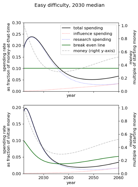
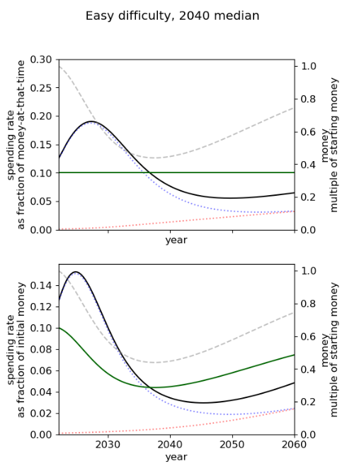
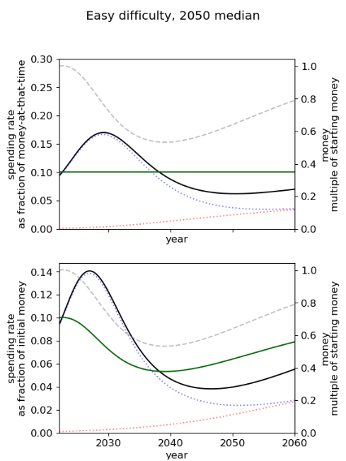
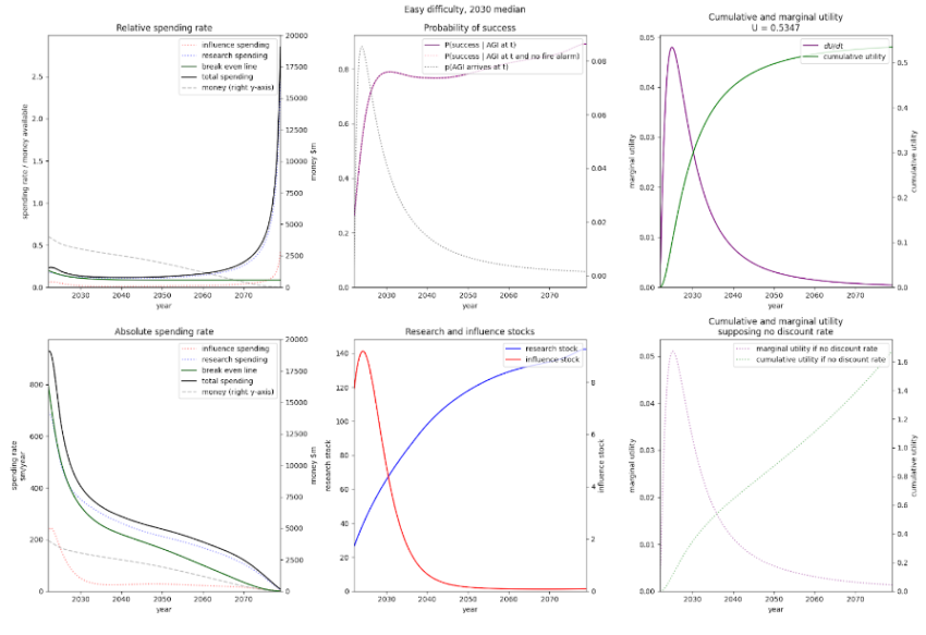
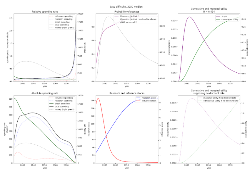
| Easy55 | Easy difficulty 2030 median56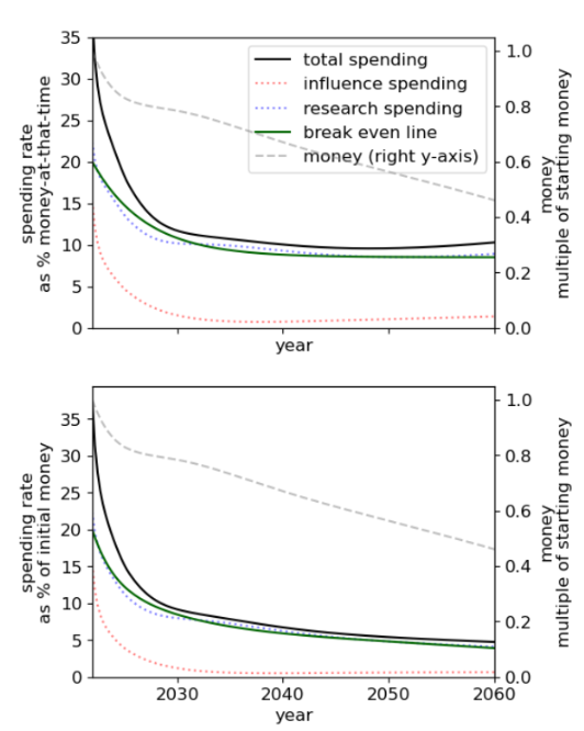 |
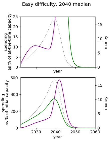
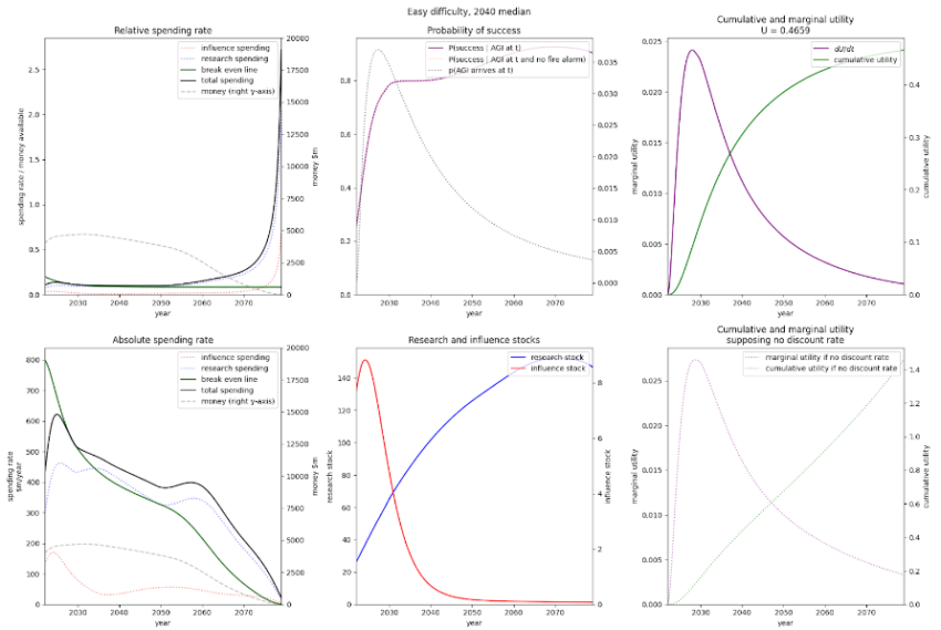
Easy difficulty 2040 median
|
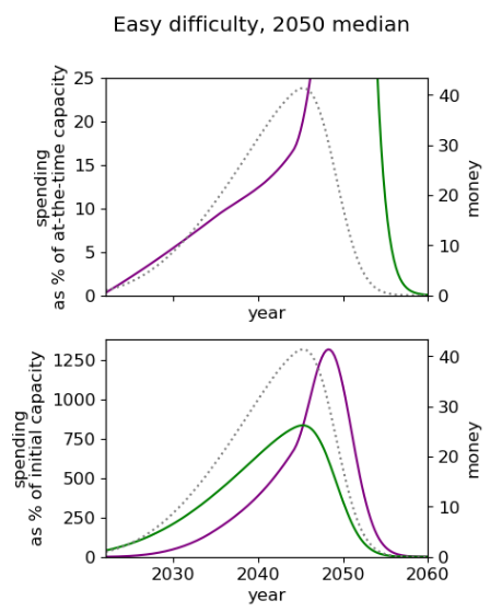
Easy difficulty 2050 median
|
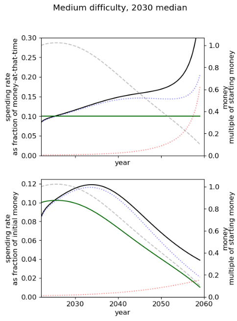
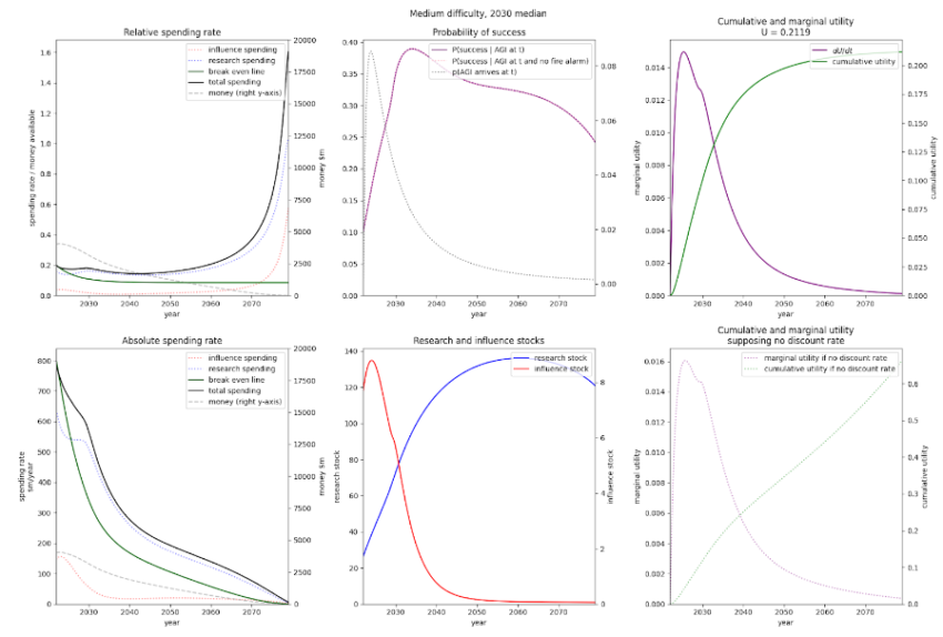
| Medium57 | Medium difficulty 2030 median
|
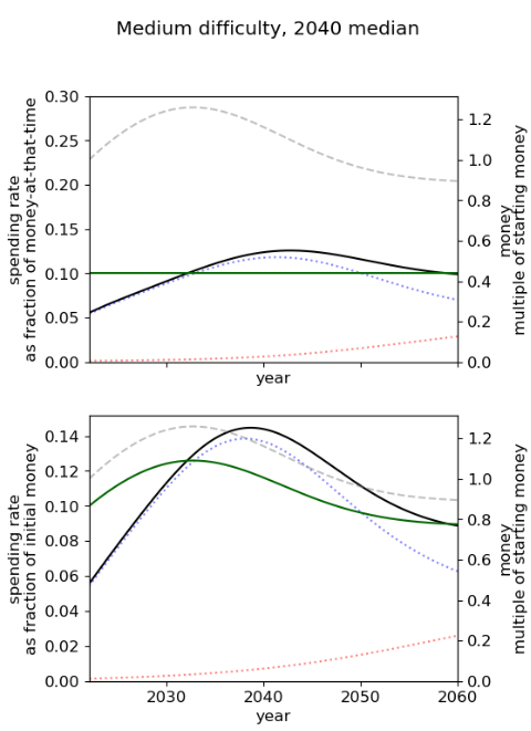
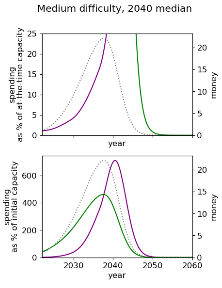
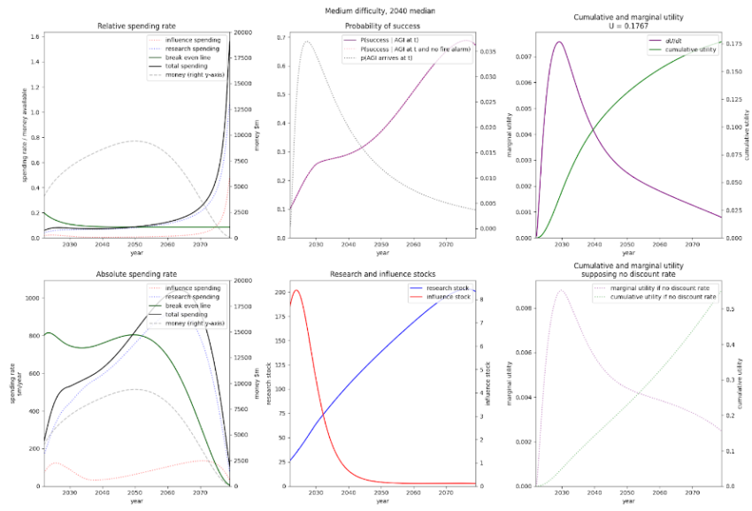
Medium difficulty 2040 median
|
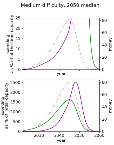
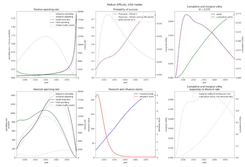
Medium difficulty 2050 median
|
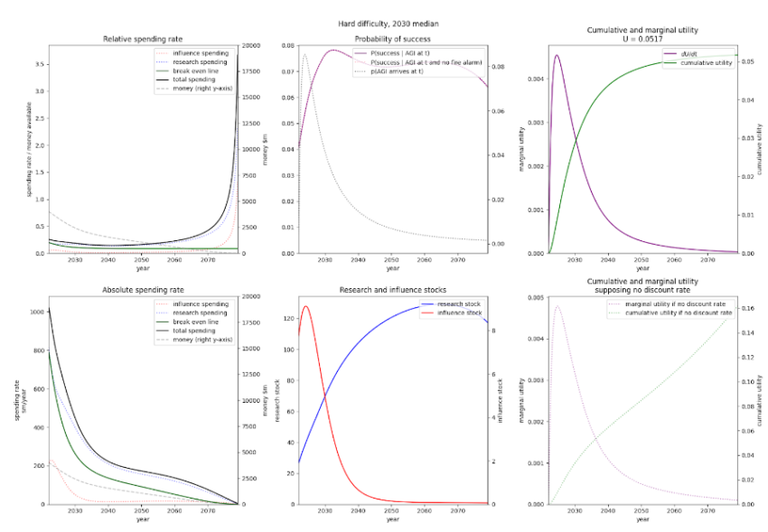
| Hard58 | Hard difficulty 2030 median
|
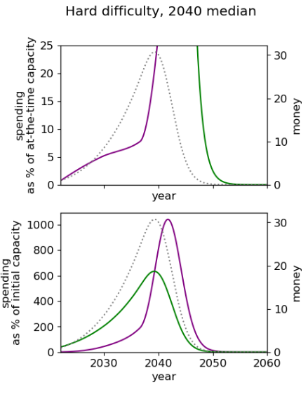
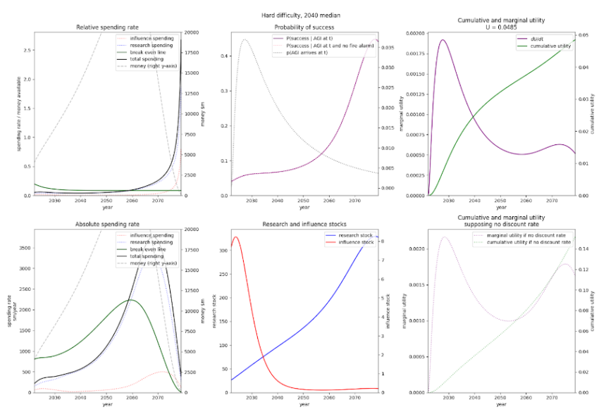
Hard difficulty 2040 median
|
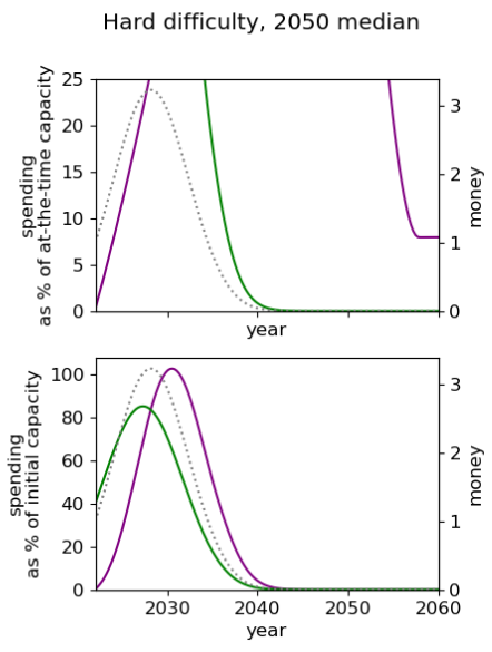
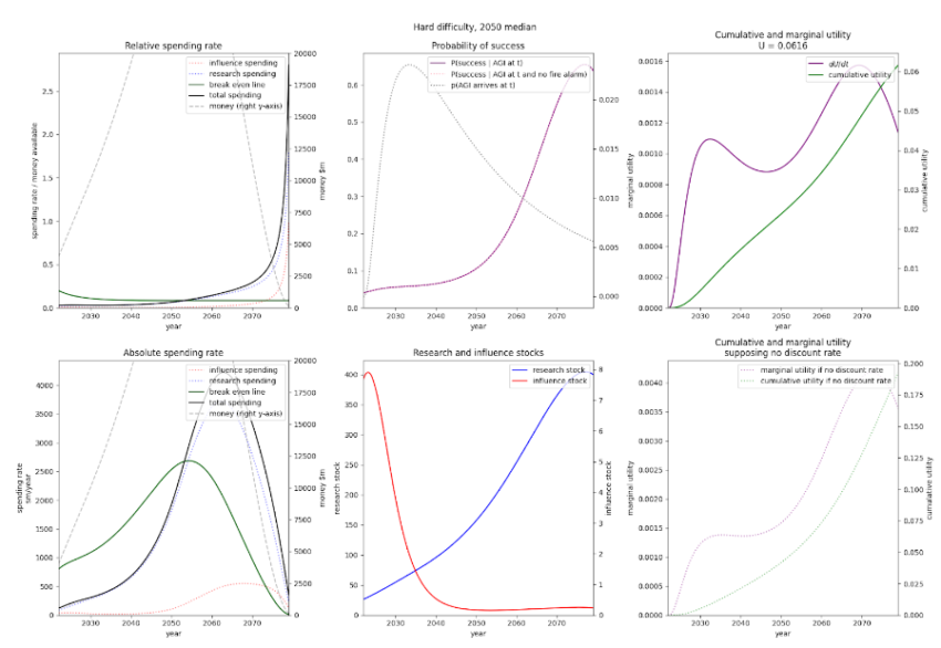
Hard difficulty 2050 median
|
|
How much better the optimal spending schedule is compared to the 2%+2% constant spending schedule (within-model lower bound)59 |
|||
|
Median AGI |
|||
| 2030 | 2040 | 2050 | |
| Easy | 37.6% | 18.4% | 11.8% |
| Medium | 39.3% | 14.9% | 12.0% |
| Hard | 12.3% | 5.85% | 1.55% |
Some of the critical limitations of our model include: poorly modelling exogenous research, which is particularly important for those with longer timelines, and many parts of the model - such as diminishing returns - remaining constant over time.
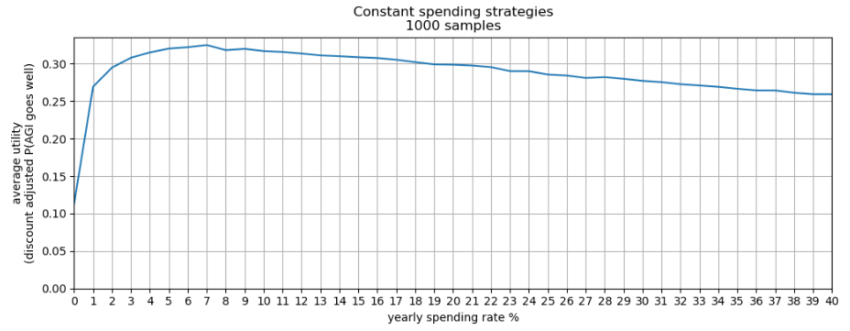
Further, we find that robust spending strategies - those that work in a wide variety of worlds - also support a higher spending rate. We show the results of a Monte Carlo simulation in the appendix60.
Introduction
Humanity might be living at a hinge moment in history (MacAskill, 2020). This is partly due to the unusually high level of existential risks (Ord, 2020) and, in particular, the significant probability that humanity will build artificial general intelligence (AGI) in the next decades (Cotra, 2022). More specifically, AGI is likely to make up for a large fraction of extinction risks in the present and next decades (Cotra, 2022) and stands as a strong candidate to influence the long-term future. Indeed, AGI might play a particularly important role in the long-term trajectory change of Earth-originating life by increasing the chance of a flourishing future (Bostrom, 2008) and reducing the risks of large amounts of disvalue (Gloor, 2016).
Philanthropic organisations aligned with effective altruism principles such as the FTX Foundation and Open Philanthropy play a crucial role in reducing AI risks by optimally allocating funding to organisations that produce research, technologies and influence to reduce risks from artificial intelligence. Figuring out the optimal funding schedule is particularly salient now with the risk of AI timelines under 10 years (Kokotajlo, 2022), and the substantial growth in effective altruism (EA) funding roughly estimated at 37% per year from 2015 to 2021 for a total endowment of about 46B$ by then end of 2021 (Todd, 2021).
Previous work has emphasised the need to invest now to spend more later due to low discount rates (Hoeijmakers, 2020, Dickens 2020). This situation corresponds to a “patient philanthropist”. Research has modelled the optimal spending schedule a patient philanthropist should follow if they face constant interest rates, diminishing returns and a low discount rate accounting for existential risks (Trammell, 2021, Trammell 2021). Extensions of the single provider of public goods model allowed for the rate of existential risks to be time-dependent (Alaya, 2021) and to include a trade-off between labour and capital where labour accounts for movement building and direct work (Sempere, Trammell 2021). Some models also discussed the trade-off between economic growth and existential risks by modelling the dynamics between safety technology and consumption technology with an endogenous growth (Aschenbrenner, 2020) and an exogenous growth model (Trammell, 2021).
Without more specific quantitative models taking into account AI timelines, growth in funding, progress in AI safety and the difficulty of building safe AI, previous estimates of a spending schedule of just over 1% per year (Todd 2021, MacAskill 2022) are at risk of underperforming the optimal spending schedule by as much as 40%.
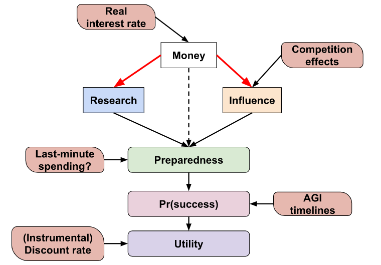
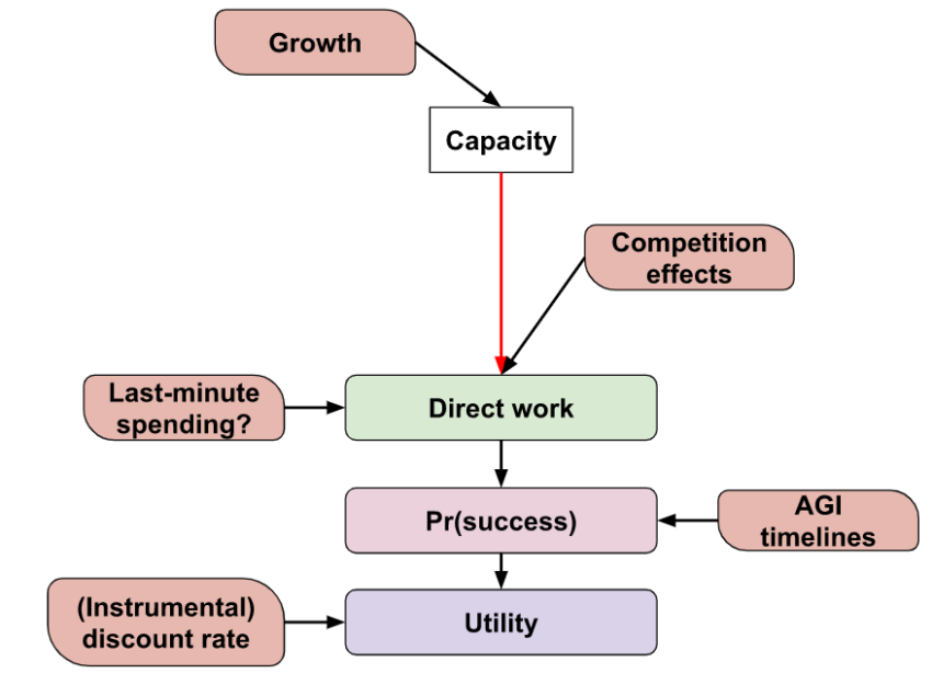
In this work, we consider a philanthropist or philanthropic organisation maximising the probability of humanity building safe AI. The philanthropist spends money to increase the stock of AI safety research and influence over AI development which translates into increasing the probability of successfully aligning AI or avoiding large amounts of disvalue. Our model takes into account AI timelines, the growth of capital committed to AI safety, diminishing returns in research and influence as well as the competitiveness of influencing AI development. We also allow for the possibility of a fire alarm shortly before AGI arrives. Upon “hearing” the fire alarm, the philanthropist knows the arrival time of AGI and wants to spend all of its remaining money until that time. The philanthropist also has some discount rate due to other existential risks and exogenous research that accelerate safety research.
Crucially, we have coded the model into a notebook accompanying this blog post that philanthropists and interested users can run to estimate an optimal spending schedule given their estimates of AI timelines, the difficulty of AI safety, capital growth and diminishing returns. Mathematically the problem of finding the optimal spending schedule translates into an optimal control problem giving rise to a set of nonlinear differential equations with boundary conditions that we solve numerically.
We discuss the effect of AI timelines and the difficulty of AI safety on the optimal spending schedule. Importantly, the optimal spending schedule typically ranges from 5% to 35% per year this decade, certainly above the current typical spending of EA-aligned funders. A funder should follow the most aggressive spending schedule this decade if AI timelines are short (2030) and safety is hard. An intermediate scenario yields a yearly average spending of ~12% over this decade. The optimal spending schedule typically performs between 5 to 15% better than the strategy of spending the endowment’s rate of appreciation and between 18% to 40% better than the current EA community spending at ~3% per year.
A qualitative description of the model
We suppose that a single funder controls all of the community’s funding that is earmarked for AI risk interventions and that they set the spending rate for two types of interventions: research and influence. The funder’s aim is to choose the spending schedule - how much they spend each year on each intervention - that maximises the probability that AGI goes successfully (e.g. does not lead to an existential catastrophe).
The ‘model’ is a set of equations (described in the appendix) and accompanying Colab notebook. The latter, once given inputs from the user, finds the optimal spending schedule.
Research and influence
We suppose that any spending is on either research or influence. Any money we don’t spend is saved and gains interest. As well as investing money in traditional means, the funder is able to ‘invest’ in promoting earning-to-give, which historically has been a source of a large fraction of the community’s capital.
We suppose there is a single number for each of the stocks of research and influence describing how much the community has of each61.
Research refers to the community’s ability to make AGI a success given we have complete control over the system (modulo being able to delay its deployment indefinitely). The stock of research contains AI safety technical knowledge, skilled safety researchers, and safe models that we control and can deploy. Influence describes the degree of control we have over the development of AGI, and can include ‘soft’ means such as through personal connections or ‘hard’ means such as passing policy. Both research and influence contribute to the probability we succeed and the user can input the degree to which they are ‘substitutable’.
The equations modelling the time evolution of research and influence have the following features:
- Diminishing marginal returns to spending; the returns to growth in research/influence from each additional unit of spending per year decreases.
- Appreciation or depreciation of research/influence over time. For example, our stock of research could depreciate by becoming less relevant over time as paradigms change and influence could depreciate over time if the AI developers we have influence over become less likely to develop AGI compared to another group.
- The price of one unit of research and influence changes based on how much you already have. For example, having more research may open up multiple parallelizable tracks for people to work on, decreasing the cost of research units. Conversely, once we have more research new researchers must spend increasing time catching up on existing work and so research could become more expensive.
- Influence can become more expensive over time due to competition. As other actors enter the field and also wish to influence AI and the field of AI development itself grows, one unit of spending can result in less influence.
Money
Any money we don’t spend appreciates. Historically the money committed to the effective altruism movement has grown faster than market real interest rates. The model allows for a variable real interest rate, which allows for the possibility that the growth of the effective altruism community slows.
Preparedness
We use the term preparedness at time  to describe how ‘ready’ we are if AGI arrived at time
  Preparedness is a function of research and influence: the more we have of each the more we are prepared. The user inputs the relative importance of each research and influence as well as the degree they are substitutable.
AGI fire alarm
We may find it useful to have money before AGI takeoff, particularly if we have a ‘fire alarm’ period where we know that AGI is coming soon and can spend most of it on last-minute research or influence. The model allows for such last-minute spending on research and influence, and so one’s money indirectly contributes to preparedness.
Success
The probability of success given AGI arriving in year is an S-shaped function of our preparedness. The model is not fixed to any definition of ‘success’ and could be, but is not limited to, “AGI not causing an existential catastrophe” or “AGI being aligned to human values” or “preventing AI caused s-risk”.
Since we are uncertain when AGI will arrive, the model considers AGI timelines input from the user and takes the integral of the product of {the probability of AGI arriving at time } and {the probability of success at time given AGI at time }.
The model also allows for a discount rate to account for non-AGI existential risks or catastrophes that preclude our research and influence from being useful or other factors.
The funder’s objective function, the function they wish to maximise, is the probability of making AGI go successfully.
Solving the model
The preceding qualitative description is of a collection of differential equations that describe how the numerical quantities of money, research and influence change as a function of our spending schedule. We want to find the spending schedule that maximises the objective function, the optimal spending schedule. We do this with tools from optimal control theory62. We call such a schedule the optimal spending schedule.
Results
Optimal spending scheduled when varying AGI timelines and difficulty of success
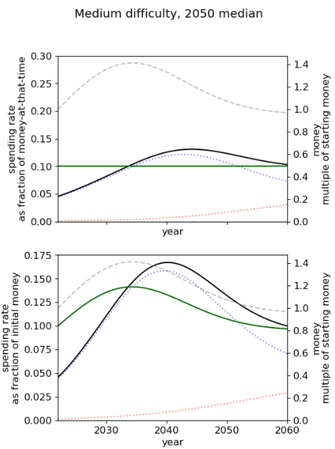
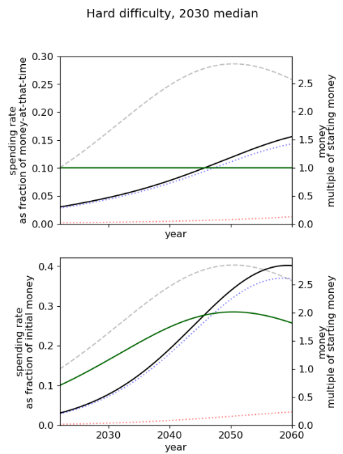
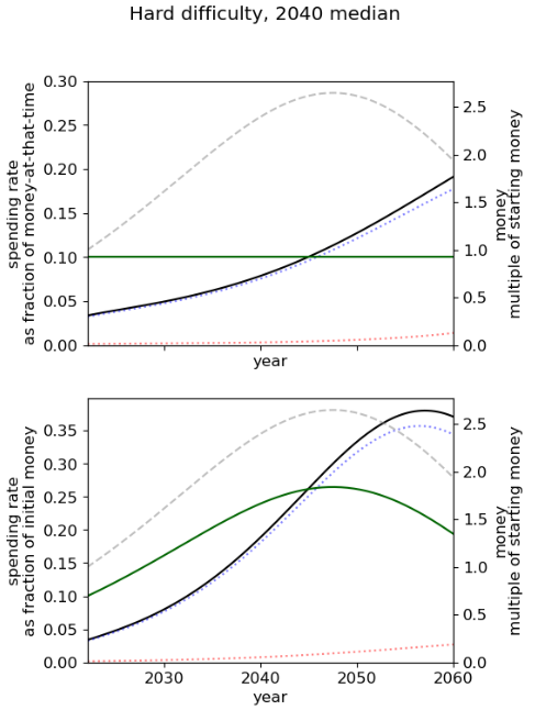
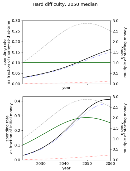
We first review the table from the start of the post, which varies AGI timelines and difficulty of an AGI success while keeping all other model inputs constant. We stress that the results are based on our guesses of the inputs (such as diminishing returns to spending) and encourage people to try the tool out themselves.
 |
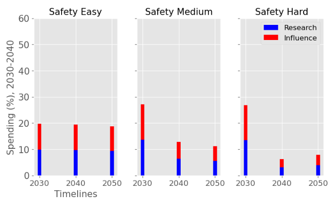 |
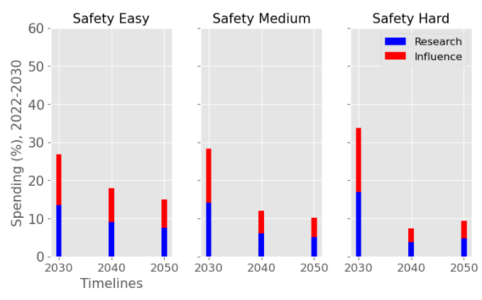
| Figure caption: Yearly optimal spending schedule averaged over this decade, 2022-2030 (left), and the next, 2030-2040 (right). For each level of AI safety difficulty (easy, medium and hard columns) and each decade we reported the average spending rates in research and influence in % of the funder’s endowment. | |
We consider our best guess for the model’s parameters as given in the appendix (see “explaining and estimating the model parameters”). We describe the effects of timelines and the difficulty of AI safety on the spending schedule in this decade (2022-2030), the effects being roughly similar in the 2030 decade.
In most future scenarios we observe that the average optimal spending schedule is substantially higher than the current EA spending rate standing at around 1-3% per year. The most conservative spending schedule happens when the difficulty of AI safety is hard with long timelines (2050) with an average spending rate of around 6.5% per year. The most aggressive spending schedule happens when AI safety is hard and timelines are short (2030) with an average funding rate of about 35% per year.
For each level of difficulty and each AI timelines, the average allocation between research and influence looks balanced. Indeed, research and influence both share roughly half of the total spending in each scenario. Looking closer at the results in the appendix (see “appendix results”), we observe that influence seems to decrease more sharply than research spending, particularly beyond the 2030 decade. This is likely caused by the sharp increase in the level of competition over AI development making units of influence more costly relative to units of research. Although we want to emphasise that the share of influence and research in the total spending schedule could easily change with different diminishing returns in research and influence parameters.
The influence of AI timelines on the optimal spending schedule varies across distinct levels of difficulty but follows a consistent trend. Roughly, with AI timelines getting longer by a decade, the funder should decrease its average funding rate by 5 to 10%, unless AI safety is hard. If AI safety is easy, a funder should spend an average of ~25% per year for short timelines (2030), down to ~18% per year with medium timelines (2040) and down to ~15% for long timelines (2050). If AI safety difficulty is medium then the spending schedule follows a similar downtrend, starting at about 30% with short timelines down to ~12% with medium timelines and down to 10% with long timelines. If AI safety is hard, the decline in spending from short to medium timelines is sharper, starting at 35% per year with short timelines down to ~8% with medium timelines and down to about 5% with long timelines.
Interestingly, conditioning on short timelines (2030), going from AI safety hard to easier difficulty decreases the spending schedule from ~35% to ~25% but conditioning on medium (204) or long (2050) timelines going from AI safety hard to easier difficulty increases the spending schedule from 6% to 18% and 9% to 15% respectively.
In summary, in most scenarios, the average optimal spending schedule in the current decade typically varies between 5% to 35% per year. With medium timelines (2040) the average spending schedule typically stays in the 10-20% range and moves up to the 20-35% range with short timelines (2030). The allocation between research and influence is balanced.
Sensitivity
In this section, we show the effect of varying one parameter (or related combination) on the optimal spending schedule. The rest of the inputs are described in the appendix. We stress again that these results are for the inputs we have chosen and encourage you to try out your own.
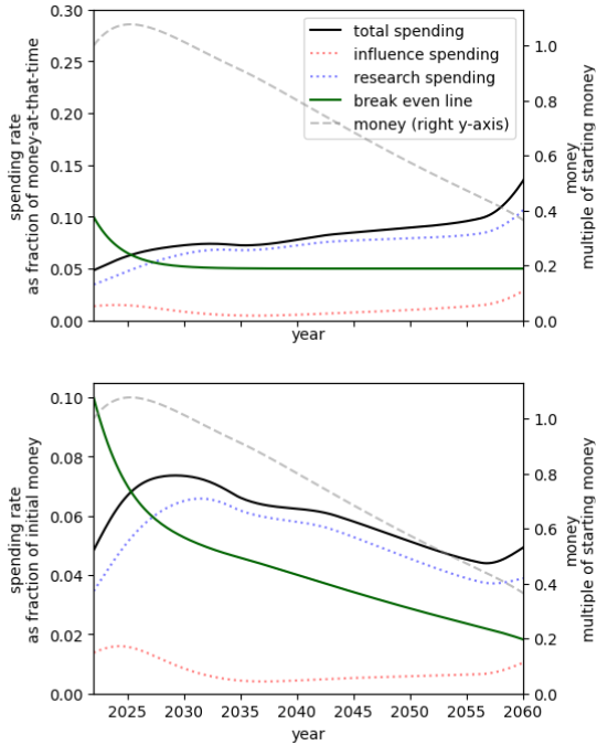
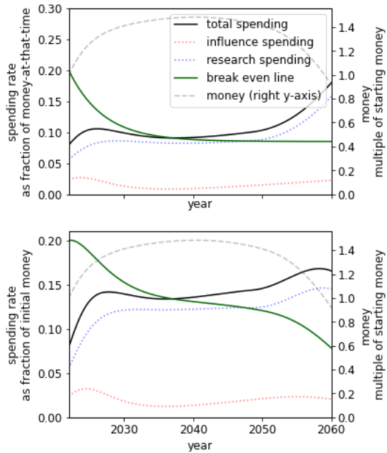
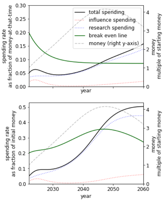
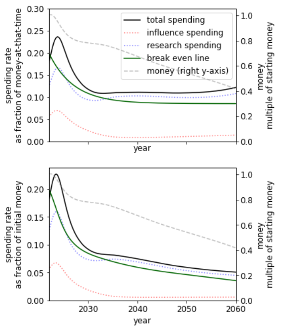
Discount rate
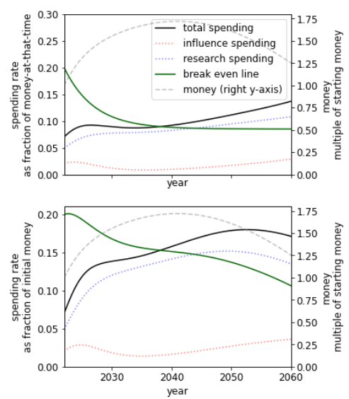
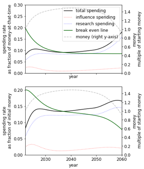
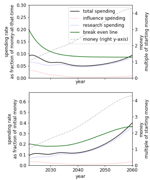
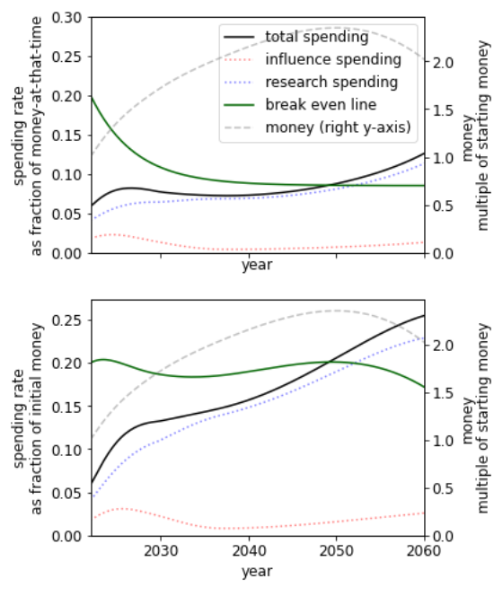
Varying just the discount rate we see that a higher discount rate implies a higher spending rate in the present.
 |
 |
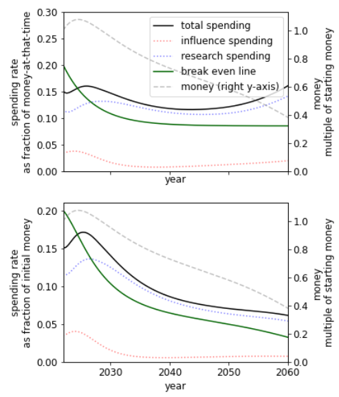 |
Low discount rate  |
Standard  |
High discount rate  |
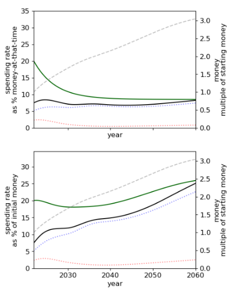
Growth rate
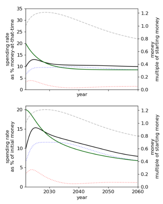
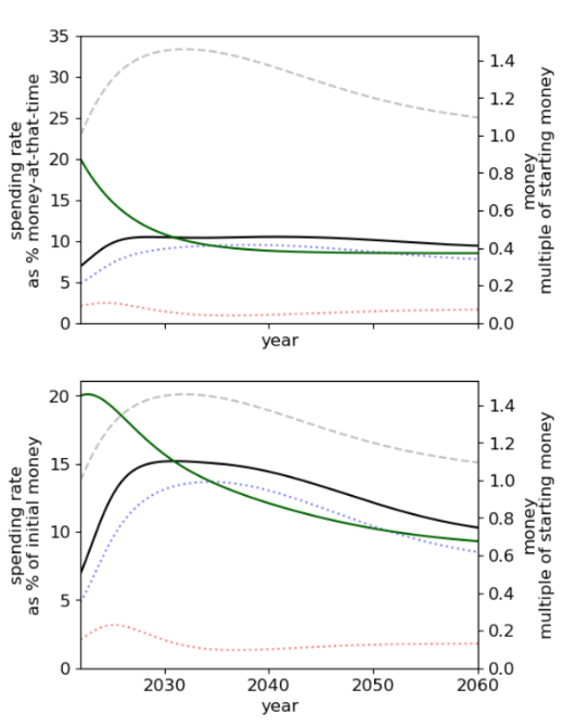
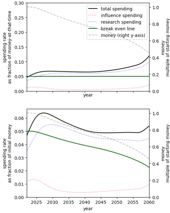
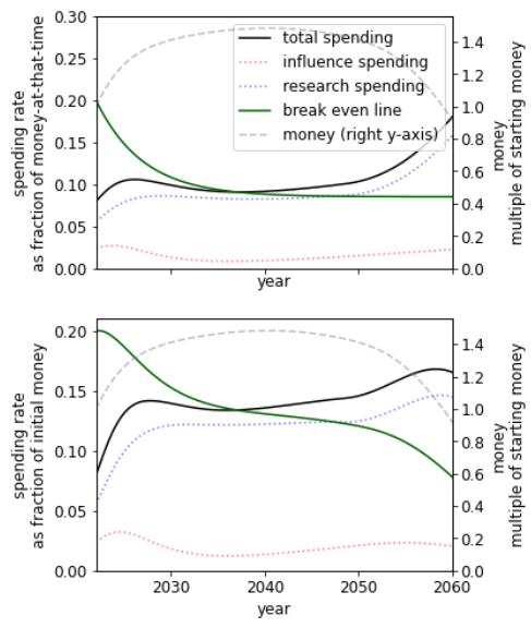
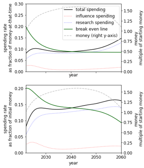
It seems plausible that the community and its capital are likely to be going through an unusually fast period of growth that will level off.63 When assuming a lower rate of growth we see that the optimal spending schedule is a lower rate, but still higher than the community’s current allocation. In particular, we should be spending faster than we are growing.
 |
 |
 |
| Highly pessimistic growth rate: 5% growth rate | Pessimistic growth rate: 10% current growth decreasing to 5% in the five years.64 | Our guess: 20% current growth decreasing to 8.5% in the next ten years.65 |
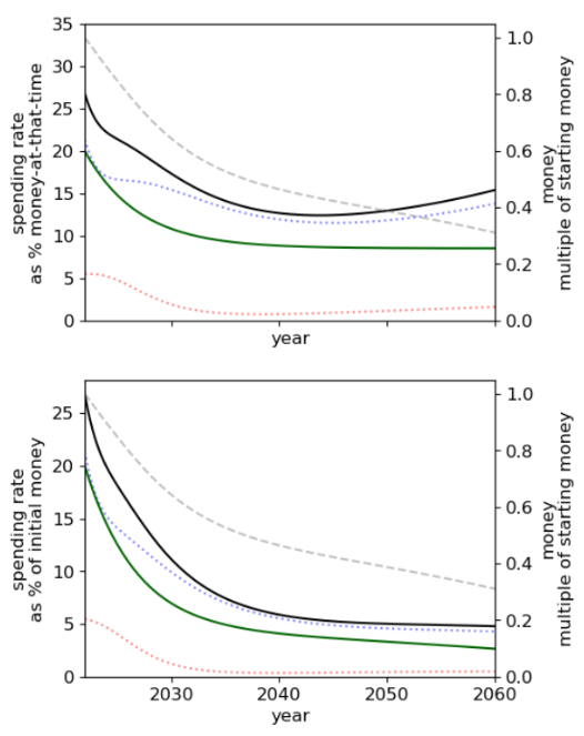
Current money committed to AGI interventions
We can compute the change in utility when the amount of funding committed to AI risk interventions changes. This is of relevance to donors interested in the marginal value of different causes, as well as philanthropic organisations that have not explicitly decided the funding for each cause area.
| Starting money multiplier | 0.001 | 0.01 | 0.1 | 0.5 | 1 | 1.1 | 1.5 | 10 |
| Absolute utility | 0.03166 | 0.044 | 0.092 | 0.219 | 0.317 | 0.332 | 0.386 | 0.668 |
| Multiple of 100% money utility | 0.098 | 0.139 | 0.290 | 0.691 | 1 | 1.047 | 1.218 | 2.107 |
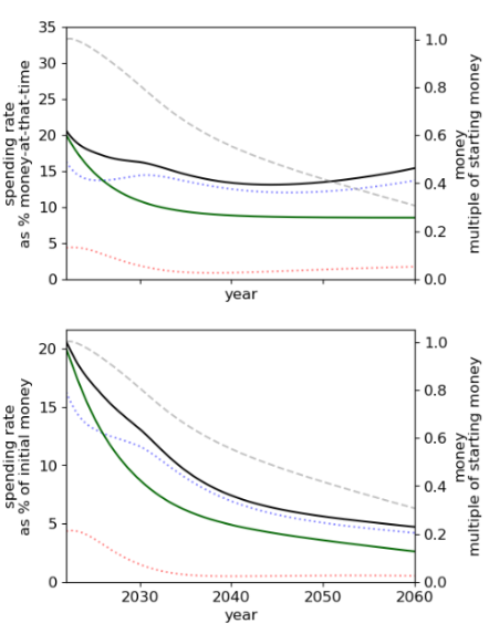
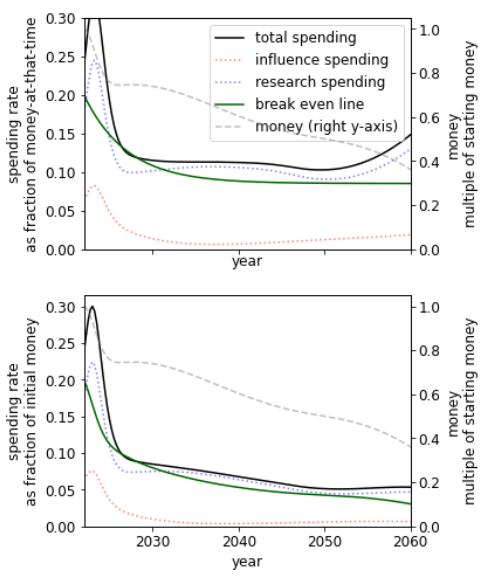
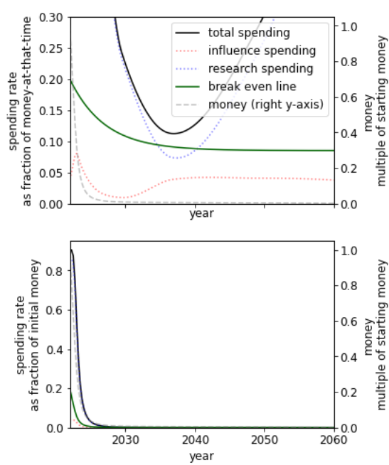
A different initial endowment has qualitative effects on the spending schedule. For example, comparing the 10% to 1000% case we see that when we have more money we - unsurprisingly - spend at a much higher rate. This result itself is sensitive to the existing stocks of research and influence.
 |
 |
| When we have 10% of our current budget of $4000m | When we have 1000% of our current budget |
The spending schedule is not independent of our initial endowment. This is primarily driven by the S-shaped success function. When we have more money, we can beeline for the steep returns of the middle of the S-shape. When we have less money, we choose to save to later reach this point.
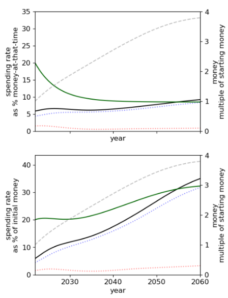
Diminishing returns
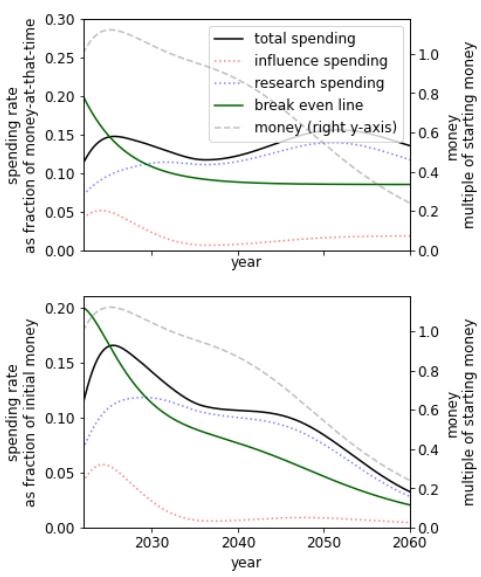
We see that, unsurprisingly, lower diminishing returns to spending suggest spending at a higher rate.
 |
 |
 |
| High diminishing returns67 | Our guess68 | Low diminishing returns69 |
Parallel vs serial research
The constant  controls whether research becomes cheaper as we accumulate more research (
 ) or more expensive (
 ). The former could describe a case where an increase in research leads to the increasing ability to parallelize research or break down problems into more easily solvable subproblems. The latter could describe a case where an increase in research leads to an increasingly bottlenecked field, where further progress depends on solving a small number of problems that are only solvable by a few people.
 |
 |
 |
Research is highly serial  |
Default ( ) ) |
Research is highly parallelizable  |
We see that in a world where research is either highly serial or parallelizable, we should be spending at a higher rate than if it is, on balance, neither. The parallelizable result is less surprising than the serial result, which we plan to explore in later work.
A more nuanced approach would use a function  such that the field can become more or less bottlenecked as it progresses and the price of research changes accordingly.
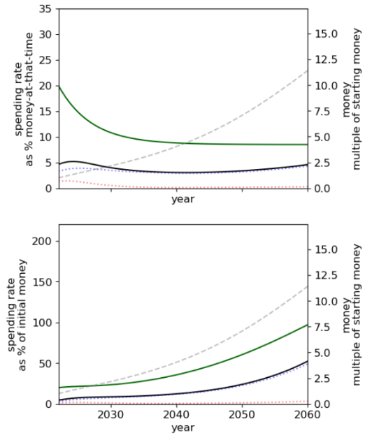
Presence of a fire alarm
Using our parameters, we find the presence of a fire alarm greatly improves our prospects and, perhaps unexpectedly, pushes the spending schedule upwards. This suggests it is both important to be able to correctly identify the point at which AGI is close and have a plan for the post-fire alarm period.
 |
 |
 |
| No fire alarm. | Short fire alarm: funders spend 10% of one’s money over six months. In this case, we get 36% more utility than no fire alarm. | Long fire alarm: funders spend 20% of one’s money over one year. In this case, we get 56% more utility than no fire alarm. |
Substitutability of research and influence
Increasing substitutability means that one (weight adjusted70) unit of research can be replaced by closer to one unit of influence to have the same level of preparedness71.
Since, by our choice of inputs, we already have much more importance-adjusted research than influence72, in the case where they are very poor substitutes we must spend at a high rate to get influence.
When research and influence are perfect substitutes since research is ‘cheaper’73 with our chosen inputs the optimum spending schedule suggests that nearly spending should be on research74.
 |
 |
 |
 |
| Research and influence are very poor substitutes75 | Research and influence are poor substitutes76 | Standard case77 | Research and influence are perfect substitutes78 |
Discussion
Some hot takes derived from the model
We make a note of some claims that are supported by the model. Since there is a large space of possible inputs we recommend the user specify their own input and not rely solely on our speculation.
The community’s current spending rate is too low
Supposing the community indefinitely spends 2% of its capital each year on research and 2% on influence, the optimal spending schedule is around 30% better in the medium timelines, medium difficulty world.
The optimal spending schedule is generally 5 to 15% better than the default strategy
Note: The default strategy is where you spend exactly the amount your money appreciates, and so your money remains constant. The greatest difference in utility comes from cases where it is optimal to spend lots of money now, for example in the (2030 median, hard difficulty) world, the optimal spending schedule is 15% better than the default strategy.
In most cases, we should not ‘wager’ on long AGI timelines when we believe AGI timelines are short
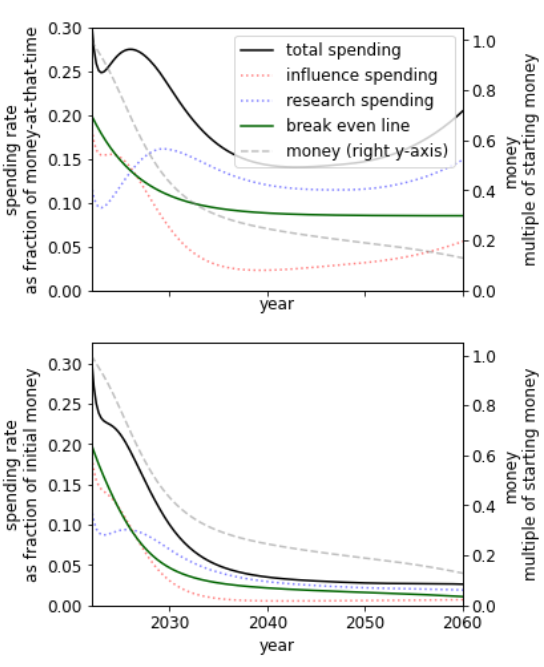
A wager is, e.g., thinking that ‘although I think AGI is more likely than not in the next t years, it is intractable to increase the probability of success in the next t years and so I should work on interventions that increase the probability of success in worlds where AGI arrives at some time  . Saving money now, even though AGI is expected sometime soon, is only occasionally recommended by the model. One case occurs with (1) a sufficiently low probability of success but steep gains to this probability after some amount of preparedness that is achievable in the next few decades, (2) a low discount rate, and either (a) that influence does not get too much more expensive over time or (b) influence is not too important.
 |
A ‘wager’ on long timelines in a case where we have 2030 AGI timelines. This case has a discount rate  , the difficulty is hard79 and the substitutability of research and influence is high80. , the difficulty is hard79 and the substitutability of research and influence is high80. |
To some extent, there is a ‘sweet spot’ on the s-shaped success curve where we wager on long timelines. If we are able to push the probability of success to a region where the slope of the s-curve is large, we should spend a high rate until we reach this point. If we are stuck on the flatter far left tail such that we remain in that region regardless of any spending we do this century to stay in that area, we should spend at a more steady rate.
In some cases, we should ‘wager’ on shorter timelines by spending at a high rate now
This trivially occurs, for example, if you have a very high discount rate. A more interesting case occurs when (1) influence is poorly substituted by research81 and either (a) influence depreciates quickly or (b) influence quickly becomes expensive.
 |
| A ‘wager’ on short timelines in a case where we have the 2050 AGI timeline. This case has ‘medium’ difficulty and low substitutability of research and influence82. |
Since the opportunity to wager on short timelines only is available now, we believe more effort should go into investigating the wager.
Limitations
We discuss the primary limitations here, and reserve some for the appendix. For each limitation, we briefly discuss how a solution would potentially change the results.
Research is endogenous
The model does not explicitly account for research produced exogenously (i.e., not as a result of our spending). For example, it is plausible that research produced in academia should be included in our preparedness.
Exogenous research can be (poorly) approximated in the current model in a few different ways.
First, one could suppose that research appreciates over time and set  . This supposes that research being done by outsiders is (directly) proportional to the research ‘we’ already have (where in this case, research done by outsiders is included in
  ). Since we model exponential appreciation, appreciation leads to a research explosion. One could slow this research explosion by supposing the appreciation term was
  for some
  .
.
Second, one could suppose that exogenous research sometimes solves the problem for us, making our own research redundant. This can be approximated by increasing the discount rate to account for the ‘risk’ that our own work is not useful. This is unrealistic in the sense that we are ‘surprised’ by some other group solving the problem.
A possible modification to the model would be to add a term  to the expression for
  that accounts for the exogenous rate of growth of research. Alternatively, one could consider a radically different model of research that considered our spending on research as simply speeding up the progress that will otherwise happen (conditioning on no global catastrophe).
We expect this is the biggest weakness of the model, especially for those with long AGI timelines. To a first approximation, if there is little exogenous research we do not need to account for it, and if there is a lot then our own spending schedule does not matter. Perhaps we might think our actions can lead us to be in either regime and our challenge is to push the world towards the latter.
AGI timelines are independent of our spending schedule
We may hope that some real-world interventions may delay the arrival of AGI, for example, passing policies to slow AI capabilities work. The model does not explicitly account for this feature of the world at all.
One extension to the model would be to change the length of the fire alarm period to be a function of the amount of influence we have. We expect this extension to imply an increase in the relative spending rate on influence. Another, more difficult extension would be to consider timelines as function  such that we can ‘push’ timelines down the road with more influence.
We expect that our ability to delay the arrival of AGI, particularly for shorter arrivals, is sufficiently minimal such that it would not significantly change the result. For longer timelines, this seems less likely to be the case.
Research and capabilities are independent.
AI capabilities and our research influence each other in the real world. For example, AI capabilities may speed up research with AI assistants. On the other hand, spending large amounts on AI interventions may draw attention to the problem and speed up AI capabilities investment.
We allow for a depreciation of research, which can be used to model research becoming outdated as capabilities advance. One can also research becoming cheaper over time83 to account for capabilities speeding up our research.
On balance, we expect this limitation to not have a large effect. If one expects a ‘slow AI takeoff’ with the opportunity to use highly capable AI tools, one can use the fire alarm feature and set the returns to research during this period to be high.
Diminishing returns, and other features, are constant
We model the returns to spending constant across time. However, actual funders seem to be bottlenecked by vetting capacity and a lack of scalable and high-return projects and so the returns to spending are likely to be high at the moment. Grantmakers can ‘seed’ projects and increase capacity such that it seems plausible that diminishing returns to spending will decrease in the future.
However, the model input only allows for constant diminishing marginal returns.
The model could be easily extended to use a function  such that marginal returns to spending on research and influence changed over time, similar to how the real interest rate
  changes over time. This would require more input from the user. Another extension could allow for the returns to be a function of how much was spent last year. However, such an extension would increase the model's complexity and decrease its usability, simplicity and (potentially) solvability.
This limitation also applies to other features of the model, such as the values and  .
.
The optimal spending schedule is not always found
Most existing applications of optimal control theory to effective altruism-relevant decision-making have used systems of differential equations that are analytically solvable and have guarantees of optimality. Our model has neither property and so we must rely on optimization methods that do not always lead to a global maximum.
Appendix
Further limitations
Many inputs are required from the user
There are around 40 free parameters that the user can set.
Many model features can be turned off. To turn off the following features:
- Variable interest rates, set
 or set
- Discount rate, set

- Appreciation or depreciation, set

- Change in price of research and influence, set

- Competition that changes the price of influence, set all competition levels to be 1 in all years.
- Only one of research or influence being necessary, set
 (for no influence) or
  (for no research) [in this case,
  does not matter]
 - Fire alarm, set the expected fraction of money spendable to 0.
One can set parameters such that the model is equivalent to like the following system
![\[\begin{array}{ccl} \dot{M}(t)&=&r\cdot M(t)-x(t)\\[0.2cm] \dot{R}(t)&=&x_R(t)^{\eta_R} \\[0.2cm] U &=& \displaystyle\int_0^\infty p(t) \cdot \dfrac{1}{1+e^{-l(R(t)- R_0)}} dt \end{array}\]](https://longtermrisk.org/wp-content/ql-cache/quicklatex.com-19068bcb479721ef05c883640bfd7a1f_l3.png "Rendered by QuickLaTeX.com")
Some results from this system84:
 |
 |
 |
 |
 |
 |
 |
 |
 |
Appreciation of money is continuous and endogenous
The current growth rate of our money is continuous. However, this poorly captures the case where most growth is driven by the arrival of new donors with lots of capital. Further, any growth is endogenous - it is always in proportion to our current capital  .
.
One modification would be to the model arrival time of future funders by a stochastic process, for example following a Poisson distribution. For example, take
![\[\dot{M}(t)=r(t)\cdot M(t) - x_R(t) - x_I(t) + \Phi(t),\]](https://longtermrisk.org/wp-content/ql-cache/quicklatex.com-03478a5727ea2222341da8f6ca89cb94_l3.png "Rendered by QuickLaTeX.com")
Where  can model endogenous and non-continuous growth of funding.
Following some preliminary experiments with a deterministic flux of funders, we are skeptical that this would substantially change the recommendations of the current model.
The model only maximises the probability of ‘success’ (with constraints given by keeping money and spending non-negative)
We see two potential problems with this approach.
First, one may care about spending money on things other than making AGI go well. The model does not tell you how to trade-off these outcomes. The model best fits into a portfolio approach of doing good, such as Open Philanthropy’s Worldview Diversification. Alternatively, one may attach some value to having money leftover post-AGI.
Second, there may be outcomes of intermediate utility between AGI being successful and not. A simple extension could consider some function of the probability of success. A more complex extension could consider the utility of AGI conditioned on its arrival time and our preparedness that accounts for near-miss scenarios.
Technical description
The funders have a stock of capital . This goes up in proportion to real interest at time  , and down with spending on research,
  , and spending on influence,
  .
.
![\[\dot{M}(t) = r(t)\cdot M(t) - x_R(t) -x_I(t)\]](https://longtermrisk.org/wp-content/ql-cache/quicklatex.com-9f06edc704d9768ba8fb2c6071354035_l3.png "Rendered by QuickLaTeX.com")
The funders have a stock of research which goes up with spending on research and can depreciate over time.
![\[\dot{R}(t) = x_R(t)^{\eta_R}\cdot R(t)^{\alpha_R}+\lambda_R R(t)\]](https://longtermrisk.org/wp-content/ql-cache/quicklatex.com-a9824085875fd70deb567d87e08cef21_l3.png "Rendered by QuickLaTeX.com")
Where
 is the marginal returns to spending on research
- is the increase or decrease in efficiency of spending due to the existing stock of research
 is the rate of appreciation of the stock of research
Similarly, funders have a stock of influence  which obeys
![\[\dot{I}(t) = x_I(t)^{\eta_I}\cdot I(t)^{\alpha_I} c(t)-\lambda_I I(t)\]](https://longtermrisk.org/wp-content/ql-cache/quicklatex.com-b1216f2d8404596c8293ec8e968c0ede_l3.png "Rendered by QuickLaTeX.com")
With constants mutatis mutandis from the research stock case and  describes how the influence gained per unit money changes over time due to competition effects. That is, over time as the field of AGI influencers crowd each unit of influence can be more expensive.
Fire alarm
We allow for the existence of an AGI fire alarm which tells us that AGI is exactly  years away and that we can spend fraction
  of our money on research and influence.
We write  and
and  for the amount of research and influence we have in expectation at AGI take-off if the fire alarm occurred at time . Within the fire alarm period, we suppose that
- we spend constant amounts on research and influence
- There is no appreciation or depreciation
- We have
 which can be different from their pre-fire alarm values.
The first and second assumptions allow for analytical expression for as a function of and .
We write  for the constant spending rate on research post-fire alarm. We take
  where
where  is the fraction of post fire-alarm spending. The system
![\[\tilde{R'}(\tau) =y_R^{\eta_{R, FA}}\cdot \tilde{R}(\tau)^{\alpha_{R, FA}} ,\, \tilde{R}(0) = R(t)\]](https://longtermrisk.org/wp-content/ql-cache/quicklatex.com-da18f556e285b448049e86610f5bf203_l3.png "Rendered by QuickLaTeX.com")
has an analytical solution and we take 
Similarly for research we take  and system
![\[\tilde{I}(\tau) = y_I^{\eta_{I,FA}}\cdot \tilde{I}(\tau)^{\alpha_{I,FA}}\cdot \tilde{c}(t), \, \tilde{I}(0) = I(t)\]](https://longtermrisk.org/wp-content/ql-cache/quicklatex.com-343d39bd49b64341f36d836bf1da7f98_l3.png "Rendered by QuickLaTeX.com")
Where  is the competition factor at the start of the fire alarm period and is chosen by the user to either be a constant or function of . Note that is a constant in the differential equation, so the system has an analytical solution of the research system above. Again we take
  . Note that the user can state that no fire alarm occurs; setting the
  implies
  and so
  and so
  .
.
Preparedness and success
Our preparedness  is given by
![\[S(t) :=(\gamma \cdot\hat{R}(t)^{\rho}+(1-\gamma)\cdot \hat{I}(t)^{\rho})^{1/\rho}\]](https://longtermrisk.org/wp-content/ql-cache/quicklatex.com-8cc11f5ded916d79033d88c1cb8d1883_l3.png "Rendered by QuickLaTeX.com")
Preparedness is the constant elasticity of the substitution production function of  and
and  where the user chooses
  and .
and .
Conditioning on AGI happening at time , we take the probability of AGI being safe as
![\[Q(t) := 1+e^{-l\cdot(S-S_0)}\]](https://longtermrisk.org/wp-content/ql-cache/quicklatex.com-e500fe032212fd67f589ae828585d56d_l3.png "Rendered by QuickLaTeX.com")
This is a logistic function with constants  and
and  determined by the user’s beliefs about the difficulty of making AGI safe.
Our objective is to maximize the probability that AGI is safe. We have an objective function
![\[U = \int_0^{\infty}Q(t)\cdot p(t)\cdot e^{-dt} dt\]](https://longtermrisk.org/wp-content/ql-cache/quicklatex.com-52155ad3cd1677f5a236e56cde88d629_l3.png "Rendered by QuickLaTeX.com")
Where  is the user’s AGI timelines and
  is some discount rate.
We have initial conditions 
Solving the model
We apply standard optimal control theory results.
We have Hamiltonian
![\[H(t)=Q(t)\cdot p(t)\cdot e^{-dt}+v_M(t)\cdot \dot{M}(t)+v_R(t)\cdot \dot{R}(t)+v_I(t)\cdot \dot{I}(t)\]](https://longtermrisk.org/wp-content/ql-cache/quicklatex.com-6825b3baa4f191f0ef1ca6461c2acdcd_l3.png "Rendered by QuickLaTeX.com")
Where  are the costate variables.
The optimal spending schedule, if it exists, necessarily follows


We solve this boundary value problem using SciPy’s solve_bvp function and apply further optimisation methods to avoid local optima.
Model guide
The model is a Python Notebook accessible on Google Colaboratory here.
Any cells that contain “User guide” are for assisting with the running of the notebook.
Below the initial instructions, you will find the user input parameters.
In the next section of this document we describe the parameters in detail and our own guesses.
Explaining and estimating the model parameters
We discuss the parameters in the same order as in the notebook.
Note, the estimates given are from Tristan and not necessarily endorsed by Guillaume.
Epistemic status: I’ve spent at least five minutes thinking about each, sometimes no more.
AI timelines
We elicit user timelines using two points on the cumulative distribution function and fit a log-normal distribution to them.
We note Metaculus’ Date of Artificial General Intelligence community prediction: as of 2022-10-06, lower 25% 2030, median 2040 and upper 75% 2072.
Note that since our log-normal distribution is parameterised by two pairs of (year, probability by year), the three distinct Metaculus interquartile pairings will give different distributions.
Discount rate
The discount rate needs to factor in both non-AGI existential risks as well as catastrophic (but non-existential) risks that preclude our AI work from being useful or any unknown unknowns that have some per year risk.
We choose  implying an AGI success in 2100 is worth
  as much as a win today. As we discuss in the limitations section, the discount rate can also account for other people making AGI successful, though this interpretation of is not unproblematic.
Of relevance may be:
- The Metaculus forecast on World War Three before 2050, current median 21%.
- The Metaculus forecast on Human Extinction by 2100, current median 3%
- The Metaculus notebook from Tamay which synthesis Metaculus forecasts to come to median 18% of global catastrophe this century.
Our 90% confidence interval for is 
Money
Starting money
As of 2022-10-06, Forbes estimates Dustin Moskovitz and Sam Bankman Fried have wealth of $8,200m and $17,000m respectively. Todd (2021) estimates $7,100m from other sources in 2021 giving a total of $32,300m within the effective altruism community.
How much of this is committed to AI safety interventions?
Open Philanthropy has spent $157m on AI-related interventions, of approximately $1500m spent so far. Supposing that roughly 15% of all funding is committed to AGI risk interventions gives at least $4,000m.
Our 90% confidence interval is  .
.
Real interest rate
We suppose that we are currently at some interest rate
 .
.Supposing the movement had $10,000m in 2015 and $32,300 in mid-2022, money in the effective altruism community has grown 21% per year.
We take  . Our 90% confidence interval is
  .
.
Historical S&P returns are around 8.5%. There are reasons to think the long-term rate may be higher - such as increase in growth due to AI capabilities - or lower - there is a selection bias in choosing a successful index. We take  . Our 90% confidence interval is
  .
.
 is the rate at which the real interest rate moves from
  to
to Our 90% confidence interval is  .
.
Research and influence
Marginal returns to spending
Influence
The constant  controls the marginal returns to spending on influence. For
  we receive diminishing marginal returns.
The top  fraction of spending per year on influence leads to
  fraction of increase in growth of influence in that year. For example,
  implies the top 20% of spending leads to roughly 80% of returns i.e. the Pareto principle.
We note that influence spending can span many orders of magnitude and this suggests reason to think there are high diminishing returns (i.e. low ). For example, one community builder may cost on the order of  per year, but investing in AI labs with the purpose of influencing their decisions may cost on the order of
  per year.
We take  which implies doubling spending on influence lead to
  times more growth of influence Our 90% confidence interval is
  .
.
Research
The constant acts in the same way for research as does for influence.
We take  , which implies a doubling of research spending leads to
  times increase in research growth and that 20% of the spending in research accounts for
  of the increase in research growth.
Potential sources for estimating  include using the distribution of karma on the Alignment Forum, citations in journals or estimates of researchers’ outputs.
Our 90% confidence interval is  .
.
Change in price of the stocks when you have more
Influence
 implies that influence becomes cheaper as we get more influence. Factors that push in this direction include:
- The existence of network effects related to being trusted and having a good reputation, For example,
- It may become easier to convince other people to trust us
- We may be given access to exclusive opportunities.
- The ‘clear wins’ model of political capital
 implies that influence becomes more expensive as we get more influence. Factors that point in this direction include:
- We can run out of opportunities to gain influence or only difficult opportunities remain.
- We could be seen as suspicious for amassing power, and trust in us decreases.
For  the price is constant.
On balance, we think the former reasons outweigh the latter, and so take  . This implies a doubling of influence leads to one unit of spending on influence leading to times more growth in influence compared to one unit of spending without this doubling. Our 90% confidence interval is
  .
.
Research
The constant acts in the same way for research as
 implies that research becomes cheaper as we get more research. Factors that push in this direction include:
- Research becoming more parallelizable. For example, sub-questions are found that can be worked on with less context or more standard backgrounds.
- Attracting greater talent to the field once you have developed the field.
 implies that research becomes more expensive as we get more research. Factors that push in this direction include:
- Research becoming more serial. That is, the field is increasingly bottlenecked by progress in a few key areas.
- The costs of getting up to speed with research increase as we accumulate new research. For example, new researchers need to learn increasingly more background material before being able to contribute.
We are uncertain about the net effect of the above contributions, and so take  . Our 90% confidence interval is
  .
.
Depreciation of stocks
Influence
 controls the rate of appreciation, for
  , or depreciation, for
  , of our stock of influence. It seems very likely that
 - AGI labs we have influence over can decrease in relative importance.
- The number of AGI labs and people working on AGI increases, and so our relative influence decreases
We take  , which implies a half-life of around
  years. Our 90% confidence interval is
Research
 , of our stock of influence.
We expect research to depreciate over time. Research can depreciate by
- Becoming less relevant over time
- Be lost, forgotten or otherwise inaccessible
One intuition pump is to ask what fraction of research on current large language models will be useful if AGI does not come until 2050? We guess on the order of 1% to 30%, implying - if all our research was on large language models - a value of between  and
and  . Note that for
  , such research can be instrumentally useful for later years due to its ability to make future work cheaper by, for example, attracting new talent.
We take  . Our 90% confidence interval is
  .
.
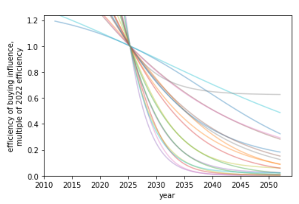
Competition effects
We allow for influence to become more expensive over time. The primary mechanism we can see is due to (a) competition with other groups that want to influence AI developers, and (b) competition within the field of AI capabilities, such that there are more organisations that could potentially develop AGI.
We suppose the influence per unit spending decreases over time following some S-shape curve, and ask for three points on this curve.
The first data point is the first year in which money was spent on influence. Since one can consider community building or spreading AI risk ideas (particularly among AI developers) as a form of influence, the earliest year of spending is unclear. We take 2015 (the first year Open Philanthopy made grants in this area). The relative cost of influence is set to 1 in this year.
We then require to further years, as well as influence per unit spending relative to the the first year of spending.
Our best guess is (2017, 0.9) - that is, in 2017 one received 90% as much influence per unit spending as one would have done in 2015- and (2022, 0.6).
The final input is the minimum influence per unit spending that will be reached be take this to be 0.02. That is, influence will eventually be  more expensive per unit that it was in 2015. Our 90% confidence interval is (0.001, 0.1).
Historical spending on research and influence
The model uses this data to calculate the quantities of research and influence we have now. Rough estimates are sufficient.
The Singularity Institute (now MIRI) was founded in 2000 and switched to work on AI safety in 2005. We take 2005 as the first year of spending on research.
Open Philanthropy has donated $243.5m to risks from AI since its first grant in the area in August 2015. We very roughly categorised each grant by research : influence fraction, and estimate that $132m has been spent on research and $111m on influence. We suppose that Open Philanthropy has made up two-thirds of the overall spending, giving totals of $198m and $167m.
We guess that the research spending, which started in 2005, has been growing at 25% per year and influence spending has been growing 40% per year since starting in 2015.
Fire alarm
By default, in the results we show, we assume no fire alarm in the model. This is achievable by setting the expected fraction of money spendable to 0. When considering the existence of a fire alarm, we take the following values.
For the fire alarm duration we ask Supposing that the leading AI lab has reached an AGI system that they are not deploying out of safety concerns, how far behind is a less safety-conscious lab? We guess this period to be half a year.
Our 90% confidence interval for this period, if it exists, is (one month, two years).
One may think that expected fraction of money spendable during the fire alarm is less than 1 for reasons such as
- Not being certain that the AGI fire alarm has gone off [though we don’t model other false positives, and are only supposing that we may worry that this actual fire alarm is a false positive]
- Limited liquidity of the capital
- Bottlenecked by transaction speeds
We take 0.1 as the expected fraction of money spendable with 90% confidence interval (0.01, 0.5).
Returns to spending during the fire alarm
During the fire alarm period, we enter a phase with no appreciation or depreciation of research or influence and a separate marginal returns to spending  and
and  can apply.
Some reasons to think  (worse returns during the fire alarm period)
- There is general panic or uncertainty around what to do and worse coordination leading to wasted effort
- The most useful technical work can only be done within highly secure environments to avoid leaks to the competitor labs
- The labs that are reaching AGI become increasingly averse to being influenced from the outside, since there may be more bad actors targeting them.
- People may be less incentivised by money if they believe AGI is near.
Some reasons to think the  (better returns during the fire alarm period)
- There are unique opportunities that arise during this period
- There is clarity over what AGI will look like.
- We can actually execute a plan that has been refined in the pre-fire-alarm period
- We can take riskier actions that would damage our reputation during the pre-fire alarm period.
- Some people will be more motivated to work harder
- Some people will be more open to the idea of AI safety, given that capabilities are at a high level
We expect that the returns to research spending will be very low, and take  , implying that the amount of research we can do in the post-fire-alarm period is not very dependent on the money we have.
We expect that returns to influence spending will be less than in the period before, lower. We take  .
.
Change in price of the stocks when you have more
In the fire alarm phase, the cost per unit of research and influence can also change depending on the amount we already have.
We expect  and
and  . That is, during the fire alarm period it is even cheaper to get influence once you already have some than before this phase and that this effect is greater during the fire alarm period (the first inequality). In the case there is panic, it seems people will be looking for trustworthy organisations to defer to and execute a plan.
We expect  That is, during the fire alarm period the amount of existing research decreases the cost of new research.
During the fire alarm period, it seems likely that only a few highly skilled researchers - perhaps within the AI lab - will have access to the information and tools necessary to conduct further useful research. The research at this point is likely highly serial: the researchers trying to focus on the biggest problems. Existing research may allow these few researchers to build on existing work effectively.
We take both  and to be 0.3, implying that a doubling of research before the fire-alarm period increases the stock output during the fire-alarm period by times.
Competition during the fire alarm period
Preparedness and probability of success
Preparedness
Preparedness at time is a function of the fire-alarm adjusted research and influence that takes two parameters, the share parameter that controls the relative importance of research and influence and parameter , that controls the substitutability of research and influence.
 .
.
 .
.Decreasing decreases the subsitutability of research and influence. In the limit as  , our preparedness can be entirely bottlenecked by the stock we have the least (weighted by
 gives the Cobb-Douglas production function, though to avoid a case-by-case situation in the programming, you cannot set and instead can choose value close to
  .
.
Again, we recommend picking values and running the cell to see the graph. We choose  . We think that the problem is mainly a technical problem, but in practise cannot be solved without influencing AI developers.
Probability of success
The probability of success at time
The first input is the probability of success if AGI arrived this year. That is, given our existing stocks of research and influence - this input doesn't consider any fire alarm spending. The second input determines the steepness of the S-shaped curve.
We take (10%, 0.15).
A note on the probability of success
Suppose you think we are in one the following three worlds
- World A: AGI will go certainly well, regardless of what we do
- World B: AGI might go well, and we can influence the probability it does
- World C: AGI will certainly not go well, regardless of what we do
Then, in the input you should imagine you should give your inputs as they are in your world B model. We keep the probability of success curve between 0 and 1, but one could linear transform it to be greater than the probability of success in the A world and less than the probability of success in the C world. Since the objective function is linear in the probability of success, such a transformation has no effect on the optimal spending schedule.
Alternate model
In an alternate model, we suppose the funder has a stock of things that grow  which includes things such as skills, people, some types of knowledge and trust. They can choose to spend this stock at some rate
  to produce a stock of things that depreciate
  that are immediately helpful in increasing the probability of success. This could comprise things such as the implementation of safety ideas on current systems or the product of asking for favours of AI developers or policymakers.
We say that spending capacity to create is crunching and the periods with high are crunch time.
The probability we succeed at time is a function of  which is plus any last-minute spending that occurs with a fire alarm. Specifically, it is another S-shaped curve.
Formalisation
| Time evolution of things that grow | |
| Time evolution of things that depreciate | |
| Post-fire alarm total of things that depreciate | |
| The probability of success given AGI at |
|
| Objective function |  |


Recall that is the expected fraction of money spendable post-fire alarm and is the expected duration of the fire alarm. The equation for is thus simply the result of spending at rate  for duration .
Estimating parameters
The alternate model shares the following parameters and machinery with the research-influence model
- AGI timelines,
- Discount rate,
- Growth rate
- Competition factor
- The duration of the fire alarm and expected fraction of money spendable
The new inputs include
- Diminishing returns to spending on direct work

- Depreciation of the direct work

- Probability of success as a function of our direct work
Growth rate
We expect the growth in capacity to decrease over time since some of our capacity is money and the same reasons will apply as in the former model. We suppose  , and
, and  .
.
Competition factor
The factor , which in the former model controlled how influence becomes more expensive over time, controls how the cost of doing direct work - producing - becomes more expensive over time. . Only some spending to produce is in competitive domains (such as influencing AI developers) while some is non-competitive, such as implementing safety features in state-of-the-art systems.
We suppose that has a minimum 0.5 and otherwise has the same factors as in the former research-influence model.
Diminishing returns to spending
This controls the degree of diminishing returns to ‘crunching’. For reasons similar to those given for and  in the main model, we take
  . Our 90% confidence interval is
  .
.
Depreciation of the direct work
This controls how long our crunch time activities are useful for i.e. the speed of depreciation. We take  which implies that after one
  of the direct work is still useful.
Probability of success
To derive the constants used in the S-shaped curve, we ask for the probability of success after some hypothetical where we've spent some fraction of our capacity for one year.
Our guess is that after spending half of our resources this year, we’d have a 25% chance of alignment success if AGI arrived this year. Note that this input does not account for any post-fire-alarm spending.
Results
Unsurprisingly we see that we should spend our capacity of things-that-grow most around the time we expect AGI to appear. For the 2040 and 2050 timelines, this implies spending very little on things that depreciate, up to around 3% a year. For 2030 timelines, we should be spending between 5 and 10% of our capacity each year on ‘crunching’ for the arrival of AGI. Further, for all results, we begin maximum crunching after the modal AGI arrival date, which is understandable while the rate of growth of the movement is greater than the rate of decrease in probability of AGI (times the discount factor).
This result is relatively sensitive to the probability we think AGI will appear in the next few years. We fit a log-normal distribution to the AGI timeline with  which leads to being small for the next few years. Considering a probability distribution that gave some weight to AGI in the next few years would inevitably imply a higher initial spending rate, though likely a similar overall spending schedule in sufficiently many years time.
| Median AGI arrival | |||
| Difficulty of AGI success | 203085 | 204086 | 205087 |
| Easy88 | 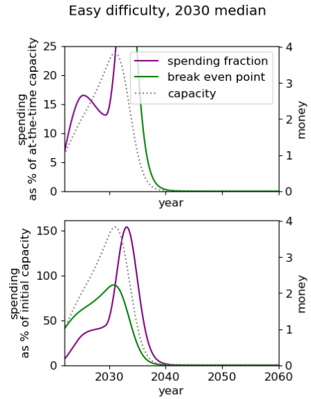 |
 |
 |
| Medium89 | 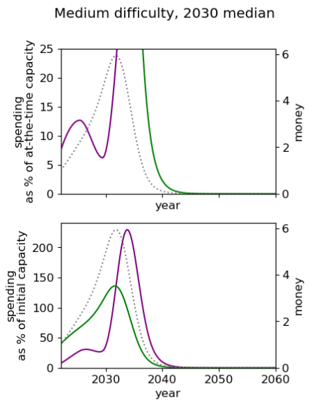 |
 |
 |
| Hard90 | 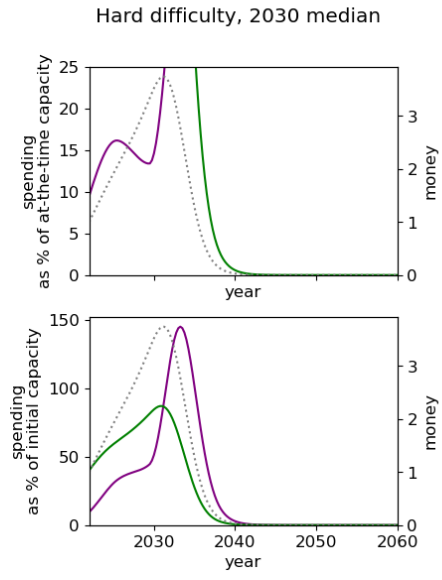 |
 |
 |
Limitations
Many of the limitations we describe apply to both models.
For example, there is no exogenous increase in which we may expect if other actors' work on AI risk at some time in the future. One could, for example, adjust such that spending on direct work receives more units of per unit spending in the future due to others' also working on the problem.
Like the first model, our work and AI capabilities are independent. One could, again, use to model direct work becoming cheaper as time goes on and new AI capabilities are developed.
Full results from the nine cases
 |
 |
 |
 |
 |
 |
 |
 |
 |
Robust spending schedules by Monte Carlo simulation
Added 2022-11-29, see discussion here
Here I consider the most robust spending policies and supposes uncertainty over nearly all parameters in the main model91, rather than point-estimates. I find that the community’s current spending rate on AI risk interventions is too low.
My distributions over the the model parameters imply that
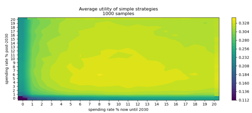
- Of all fixed spending schedules (i.e. to spend X% of your capital per year92), the best strategy is to spend 4-6% per year.
- Of all simple spending schedules that consider two regimes: now until 2030, 2030 onwards, the best strategy is to spend ~8% per year until 2030, and ~6% afterwards.
I recommend entering your own distributions for the parameters in the Python notebook here93. Further, these preliminary results use few samples: more reliable results would be obtained with more samples (and more computing time).
I allow for post-fire-alarm spending (i.e., we are certain AGI is soon and so can spend some fraction of our capital). Without this feature, the optimal schedules would likely recommend a greater spending rate.
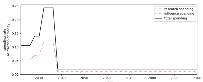 |
| The results from a simple optimiser94, when allowing for four spending regimes: 2022-2027, 2027-2032, 2032-2037 and 2037 onwards. This result should not be taken too seriously: more samples should be used, the optimiser runs for a greater number of steps and more intervals used. As with other results, this is contingent on the distributions of parameters. |
Some notes
- The system of equations - describing how a funder’s spending on AI risk interventions change the probability of AGI going well - are unchanged from the main model.
- This version of the model randomly generates the real interest, based on user inputs. So, for example, one’s capital can go down.
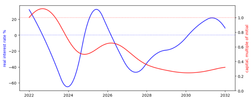 , cherry picked to show how our capital can go down significantly. See here for 100 unbiased samples of
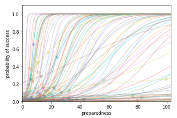
This short extension started due to a conversation with David Field and comment from Vasco Grilo; I’m grateful to both for the suggestion.
Author contributions
Tristan and Guillaume defined the problem, designed the model and its numerical resolution, interpreted the results, wrote and reviewed the article. Tristan coded the Python notebook and carried out the numerical computations with feedback from Guillaume. Tristan designed, coded, solved the alternate model and interpreted its results.
Acknowledgements
We’d both like to thank Lennart Stern and Daniel Kokotajlo for their comments and guidance during the project. We’re grateful to John Mori for comments.
Guillaume thanks the SERI summer fellowship 2021 where this project started with some excellent mentorship from Lennart Stern, the CEEALAR organisation for a stimulating working and living environment during the summer 2021 and the CLR for providing funding to support part-time working with Tristan to make substantial progress on this project.
- Todd (2021) claims 1% donated per year for the whole effective altruism community. The Open Philanthropy project spent \$80m in 2021 on AI risk interventions. In 2021 they had approximately \$17.8b committed. Supposing that at least one sixth of their budget is committed to AI risk interventions, this gives a spending rate of at most 2.6%. The FTX Future Fund has granted around \$31m on AI risk interventions since starting over a year ago. Supposing at least one tenth of their budget is committed to AI risk interventions, this gives a spending rate of at most \$31m/(\$16,600m /10) = 1.9% per year. For the AI s-risk community, the figure is around 3%.
- This is true when supposing a 4% constant spending rate, which is an overestimate of current spending but maybe underestimating future spending.
- The second model requires us to split activities into capacity growing and capacity shrinking that increase our probability of success whereas the first model talks concretely about the spending rate of money.
- The values chosen are discussed here.
- 25% AGI by 2027, 50% 2030
- 50% AGI by AGI by 2040, 75% by 2060
- 50% AGI by 2050, 75% by 2075
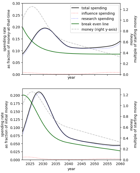
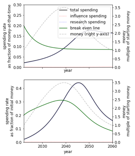
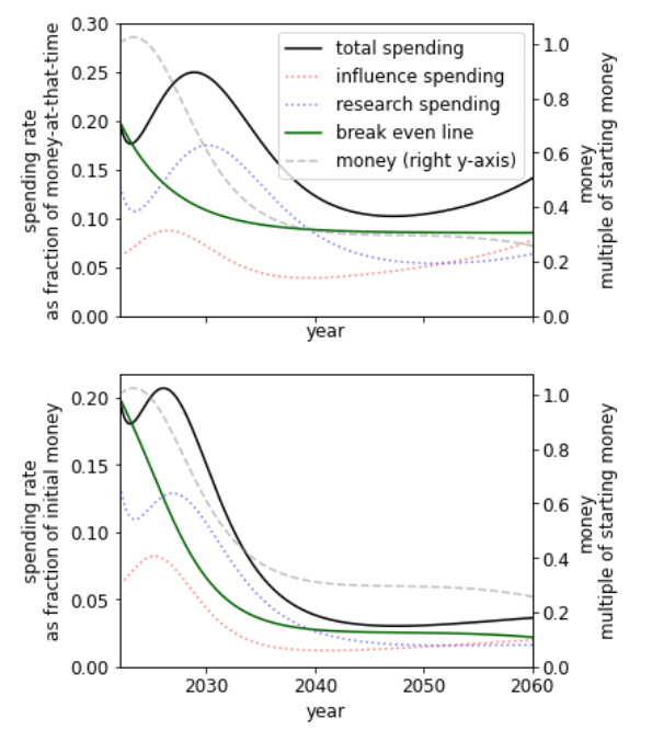
- The easy case is operationalised by the inputs in the model: Probability of success if AGI this year = 25%, and $l=0.20$. The $l$ term describes the steepness of the s-shaped curve of success.
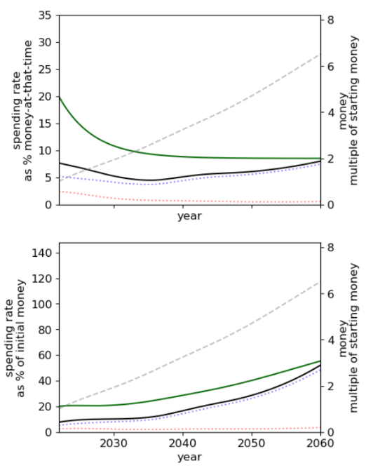
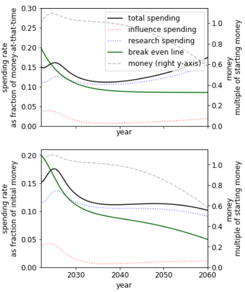
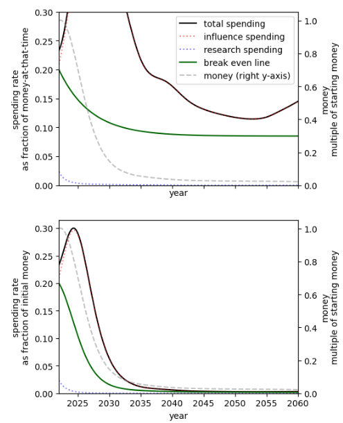
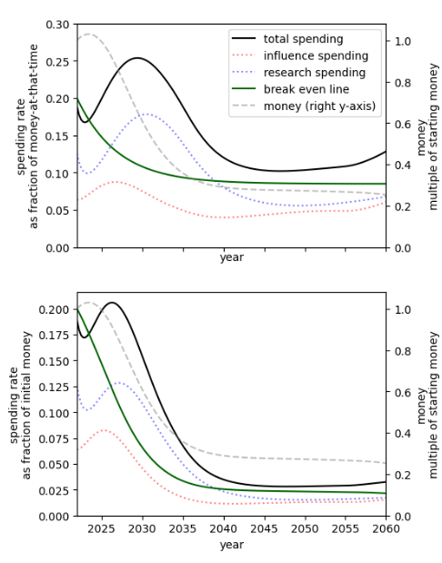
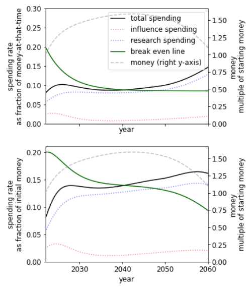
- The “break even line” is the maximum rate at which the funder can spend and still have their money increase.
- Probability of success if AGI this year = 10%, and $l=0.10$
- p(success if AGI this year) = 4%, and $l=0.05$
- This is a lower bound for two reasons: first, there may be spending schedules better than those that we present. Second, we calculate the utility of the 4% strategy for an arbitrarily long time horizon whereas we compute the optimal spending schedules within the year 2100.
- Added post-publication on 2022-11-29
- We use semi-arbitrary units of ‘quality-adjusted relevant effort units’. We use ‘quality-adjusted’ to imply that an expert's hour of contribution is worth more than a novice’s hour of contribution. We use ‘relevant’ to discount any previously acquired research or influence that is no longer useful. We use ‘effort units’ to mostly account for the time that people have put into working on something.
- We give a more complete account in the technical description. In short, the solution is given as a numerical solution to an expanded set of differential equations.
- The opposite is also plausible if AI risk becomes increasingly salient.
- Taking $\delta=0.4$
- Taking $\delta=0.2$
- We see that even with practically no money we still achieve some utility. This is because both (1) the probability of success is non-zero when we have no research or influence, and (2) we already have some research and influence that will depreciate over time with no further spending.
- $\eta_R = 0.15, \eta_I = 0.1$
- As discussed in the appendix, this is $\eta_R =0.3 , \eta_I = 0.2$
- $\eta_R =0.45 , \eta_I = 0.3$
- This weight-adjusted is the $\gamma$ term in the constant elasticity of substitution function
- This is done by increasing $\rho$ up to 1.
- This is due to our choice of $\gamma$
- In the sense that (1) it depreciates at a lower rate (2) there are lower diminishing marginal returns.
- At a high enough spending rate one marginal unit of influence is cheaper than one marginal unit of influence due to diminishing marginal returns
- We take $\rho=-10$
- We take $\rho = 0.001$
- This has $\rho=0.3$
- This is $\rho=1$
- Probability of success if AGI is this year is 0.1%, and steepness $l=0.1$
- $\rho =0.8$
- This is $\rho$ is low, perhaps less than or equal to zero.
- We take $\rho \approx 0$, so this is the Cobb-Douglas production function
- Similar to how $c(t)$ makes influence more expensive over time.
- We have $r=0.10, \, \eta_R = 0.3, \, M_0 = 4000$
- 50% AGI by 2030, 75% by 2040
- 50% AGI by AGI by 2040, 75% by 2060
- 50% AGI by 2050, 75% by 2075
- 50% AGI success if we spent half our capacity for one year, $\kappa = 5$
- 25% AGI success if we spent half our capacity for one year, $\kappa = 3$
- 10% AGI success if we spent half our capacity for one year $\kappa =1$
- Inputs that are not considered include: historic spending on research and influence, the rate at which the real interest rate changes, the post-fire alarm returns are considered to be the same as the pre-fire alarm returns.
- And supposing a 50:50 split between spending on research and influence
- This notebook is less user-friendly than the notebook used in the main optimal spending result (though not un user friendly) - let me know if improvements to the notebook would be useful for you.
- The intermediate steps of the optimiser are here.
- Todd (2021) claims 1% donated per year for the whole effective altruism community. The Open Philanthropy project spent $80m in 2021 on AI risk interventions. In 2021 they had approximately $17.8b committed. Supposing that at least one sixth of their budget is committed to AI risk interventions, this gives a spending rate of at most 2.6%. The FTX Future Fund has granted around $31m on AI risk interventions since starting over a year ago. Supposing at least one tenth of their budget is committed to AI risk interventions, this gives a spending rate of at most $31m/($16,600m /10) = 1.9% per year. For the AI s-risk community, the figure is around 3%.
- This is true when supposing a 4% constant spending rate, which is an overestimate of current spending but maybe underestimating future spending.
- The second model requires us to split activities into capacity growing and capacity shrinking that increase our probability of success whereas the first model talks concretely about the spending rate of money.
- The values chosen are discussed here.
- 25% AGI by 2027, 50% 2030
- 50% AGI by AGI by 2040, 75% by 2060
- 50% AGI by 2050, 75% by 2075
- The easy case is operationalised by the inputs in the model: Probability of success if AGI this year = 25%, and
 . The
. The  term describes the steepness of the s-shaped curve of success.
 - The “break even line” is the maximum rate at which the funder can spend and still have their money increase.
- Probability of success if AGI this year = 10%, and

- p(success if AGI this year) = 4%, and

- This is a lower bound for two reasons: first, there may be spending schedules better than those that we present. Second, we calculate the utility of the 4% strategy for an arbitrarily long time horizon whereas we compute the optimal spending schedules within the year 2100.
- Added post-publication on 2022-11-29
- We use semi-arbitrary units of ‘quality-adjusted relevant effort units’. We use ‘quality-adjusted’ to imply that an expert's hour of contribution is worth more than a novice’s hour of contribution. We use ‘relevant’ to discount any previously acquired research or influence that is no longer useful. We use ‘effort units’ to mostly account for the time that people have put into working on something.
- We give a more complete account in the technical description. In short, the solution is given as a numerical solution to an expanded set of differential equations.
- The opposite is also plausible if AI risk becomes increasingly salient.
- Taking

- Taking
- We see that even with practically no money we still achieve some utility. This is because both (1) the probability of success is non-zero when we have no research or influence, and (2) we already have some research and influence that will depreciate over time with no further spending.

- As discussed in the appendix, this is


- This weight-adjusted is the term in the constant elasticity of substitution function
- This is done by increasing up to 1.
- This is due to our choice of
- In the sense that (1) it depreciates at a lower rate (2) there are lower diminishing marginal returns.
- At a high enough spending rate one marginal unit of influence is cheaper than one marginal unit of influence due to diminishing marginal returns
- We take

- We take

- This has
- This is

- Probability of success if AGI is this year is 0.1%, and steepness


- This is is low, perhaps less than or equal to zero.
- We take
 , so this is the Cobb-Douglas production function
 - Similar to how makes influence more expensive over time.
- We have

- 50% AGI by 2030, 75% by 2040
- 50% AGI by AGI by 2040, 75% by 2060
- 50% AGI by 2050, 75% by 2075
- 50% AGI success if we spent half our capacity for one year,

- 25% AGI success if we spent half our capacity for one year,

- 10% AGI success if we spent half our capacity for one year

- Inputs that are not considered include: historic spending on research and influence, the rate at which the real interest rate changes, the post-fire alarm returns are considered to be the same as the pre-fire alarm returns.
- And supposing a 50:50 split between spending on research and influence
- This notebook is less user-friendly than the notebook used in the main optimal spending result (though not un user friendly) - let me know if improvements to the notebook would be useful for you.
- The intermediate steps of the optimiser are here.